

How do you take a picture of a landscape? You point your camera or smartphone, focus and shoot. For astronomical pictures the procedure is not very different, although the time between pressing the shutter and completing the acquisition of the image can be very long. But how do we obtain an image from a radio telescope? First of all, as we saw in the section Electromagnetic radiation, the wavelength of radio radiation is different, so for radio radiation we must use a different detection system from the one used for visible radiation. The behaviour of electromagnetic waves is very similar across the various wavelengths, but the different energies of the photons impose a difference in the type of detectors: a photon of visible light can generate electrons in a CCD, a sensitive device mounted on all cameras and smartphones, whereas for a radio electromagnetic wave a metal bar is needed. How a radio photon is detected and recorded is illustrated in the section The acquisition chain of a radio telescope.
In this section, instead, we will deal with how we collect the radiation, and with the tricks we have developed to obtain astronomical images useful for the studies to be carried out.
Before talking about the radio telescope we must introduce some information concerning geometrical optics.
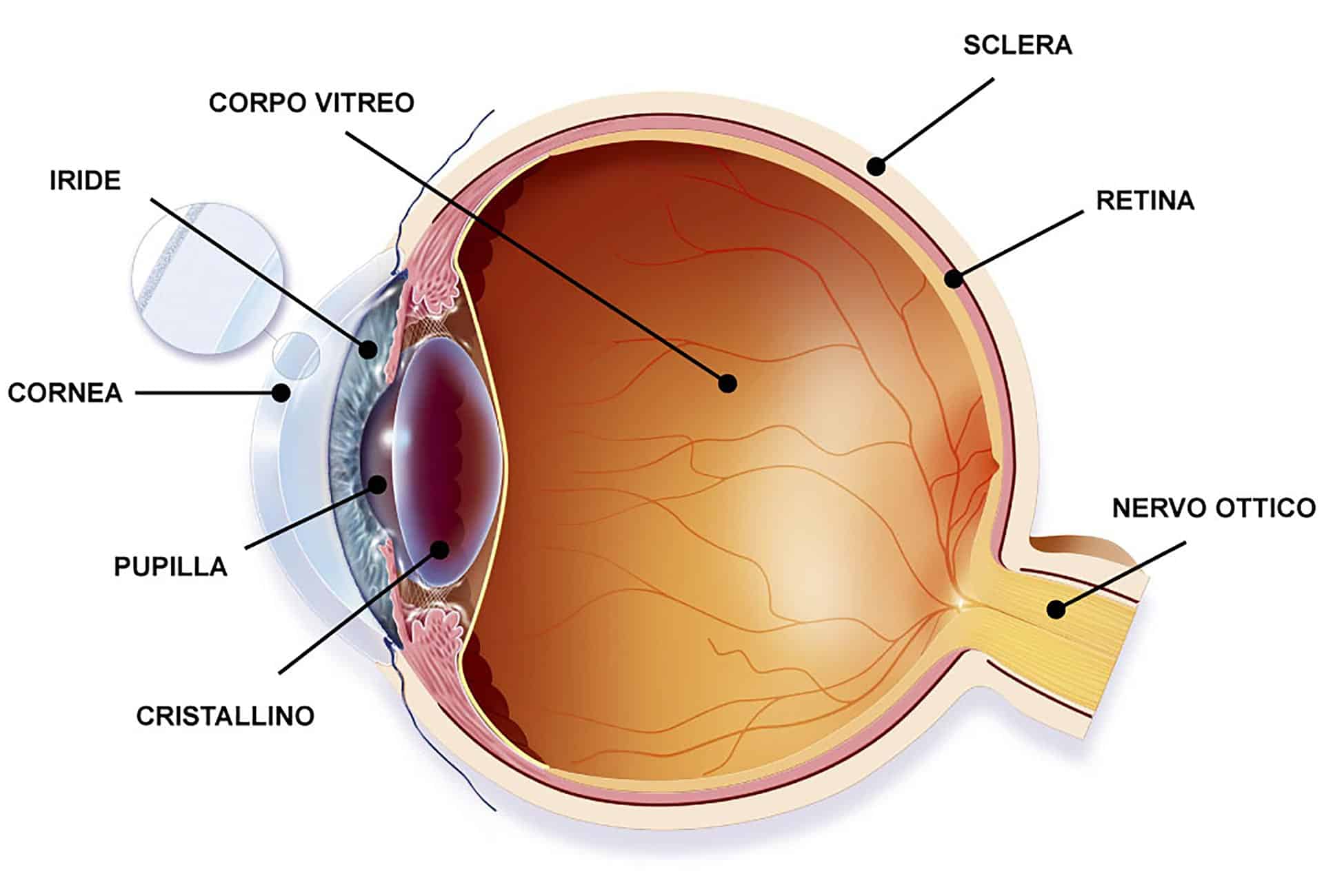
Any optical instrument, including your eyes, works because it has a "window" through which the radiation enters. Let us consider the eye first. You can see a cross-section diagram of it in fig. 1.
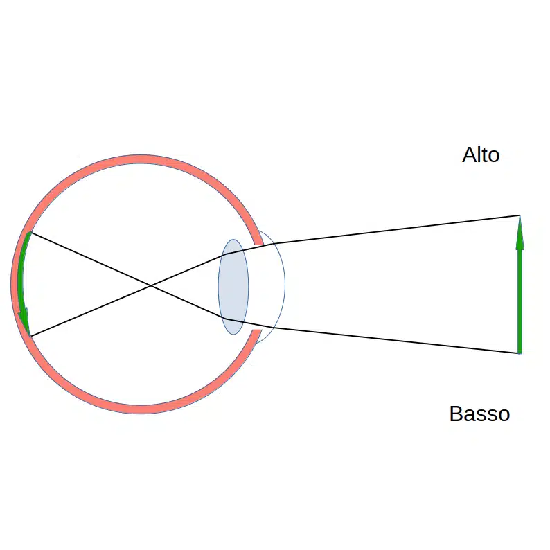
Light enters the eye through the cornea, which is the first lens to bend it; it then crosses the pupil and is immediately refracted by a lens located just behind the pupil, the crystalline lens. The focus of the cornea–crystalline system lies at about two thirds of the diameter of the eye and is arranged to be exactly the right length for the image to form on the retina. Sometimes there are vision defects that prevent the crystalline lens from doing its job properly, but let us concentrate on an eye without defects. First, let us see how an image forms on the retina. Look at fig. 2
The figure shows the optical diagram of a human eye and how an arrow pointing upwards is seen. The light rays coming from the ends of the green arrow pass through the cornea, pupil and crystalline lens and converge on the retina. The image that forms is upside down, because of the converging effect of the cornea and crystalline lens acting as lenses. The same thing happens in every direction. Since the eye has spherical symmetry, whatever direction an object extends in, the directions are inverted: in the horizontal case it is left and right that are flipped. Our brain then performs an inversion, allowing us to see reality in the same sense as we perceive up and down — from our perception of gravity and balance — and left and right, given our axial symmetry and lateralisation: we are symmetrical when divided lengthwise and we favour one of our two hands.
When we look at distant objects through a spyglass or binoculars we see them in the same way as the human eye does, flipped — although this time what bends the light in such instruments are two converging lenses, the objective and the eyepiece.
The objective plays the role of the pupil and crystalline lens; the eyepiece, placed at the right distance, does the opposite job to the objective, turning the light rays from converging back to parallel, as they were before entering the spyglass. To see this we can consider the first optical instrument designed for astronomical observation.
The telescope, as we conceive it today, was invented by Galileo Galilei by modifying the spyglass, an instrument already in use in navigation but which had never been used to magnify objects in the night sky. Galileo did not call it a telescope, but kept the original name of cannocchiale — an eyeglass shaped like a tube.
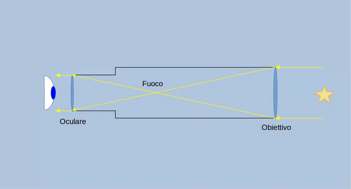
A telescope like Galileo's works as in fig. 3.
The radiation coming from the object being observed, be it a distant galaxy or a planet of our Solar System, enters the instrument through the aperture on the right and passes through the objective, which because of refraction bends the light rays until it concentrates them at a point called the focus of the lens. From that point the rays continue until they meet the eyepiece, which allows an eye placed behind it to see. The two lenses have different distances between the centre of the lens and the focus — a distance called the focal length — and the foci of the two lenses must coincide. The magnification of the telescope depends on the ratio of these distances.
This type of telescope is called a refractor, precisely because it uses the refraction of light through lenses.
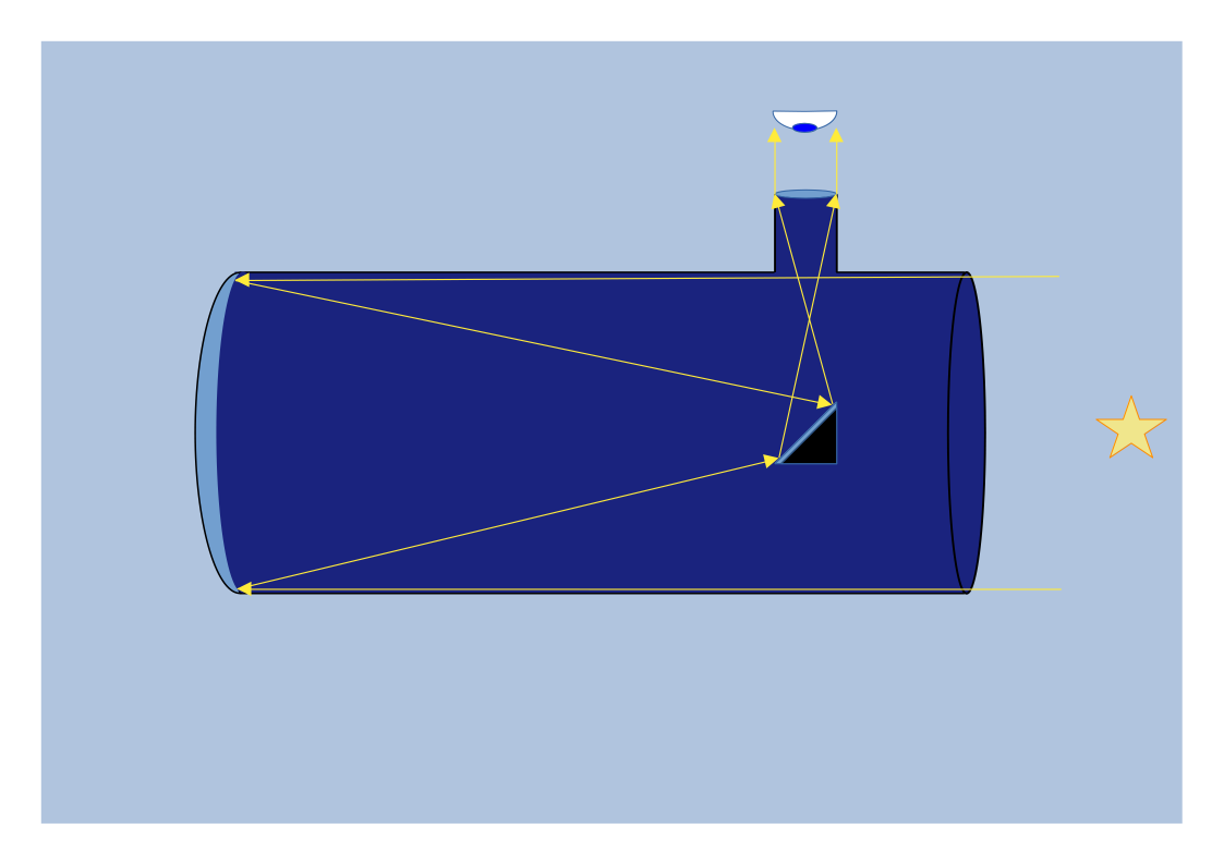
But a lens as the objective is not strictly necessary to obtain this result. The objective can in fact be replaced with a concave mirror, as seen in fig. 4.
The light rays, after striking the mirror, are reflected towards the focus of the mirror, and from there they can be reflected again and then directed to an eyepiece. The scheme you saw in fig. 4 is called Newtonian, after Isaac Newton, who developed it essentially to be able to observe through a concave mirror but in a direction different from the axis of the telescope, so that the observer would not stand between the object under study and the mirror.
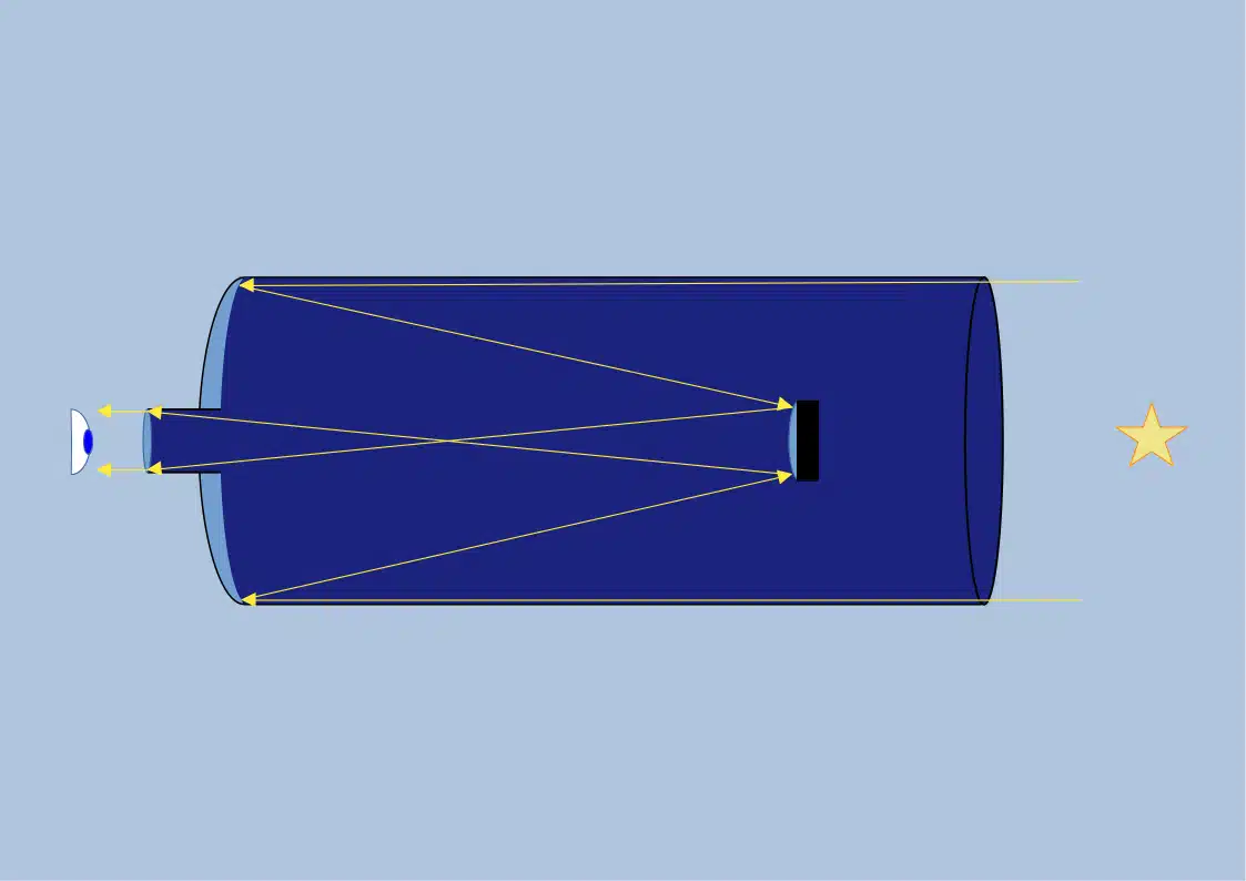
What you see in fig. 5 is a Cassegrain scheme, after Laurent Cassegrain, the French astronomer who designed it.
Here, after the concave mirror — identical to the Newtonian arrangement — there is a convex one, which reflects the radiation again towards the eyepiece. This arrangement has the merit of lengthening the focal distance. While in the Newtonian arrangement the focal length equals the focus of the primary mirror, the introduction of the secondary mirror in the Cassegrain extends the total focal length of the telescope by the whole focal length of the secondary mirror. Moreover, the Cassegrain arrangement allows the observer to be placed at the same point as the observer of a refracting telescope. A telescope that uses a mirror to concentrate the radiation is called a reflector, for the obvious reason that reflection, not refraction, is used to concentrate the radiation.
Why use a mirror instead of a lens? Because a very large lens becomes heavy and fragile. And why we need large telescopes is explained by two important characteristics of every telescope.
Sensitivity of a telescope
The amount of radiation collected by any instrument, including the eye, depends only on the area of the aperture that collects the radiation, and hence on its diameter. We can look at it this way. Suppose we want to collect rainwater and measure its amount in litres to know how much has fallen. Let us do it with a bucket, measuring the water that collects at the bottom with a graduated container. Suppose one millimetre of water rains onto the bottom of the bucket. The amount of water would be truly meagre, and if we consider the losses due to evaporation or to the few drops that cling to the bucket, we could lose an amount of water that is small indeed but comparable to the one we want to measure. Let us try the same operation with a swimming pool.
The bottom of the pool would still be covered by one millimetre of water, because the amount of rain per square metre is always the same, but one millimetre multiplied by the surface of the pool makes many litres of water, which are much more easily measured. This is the difference between an insensitive instrument and a very sensitive one: the quantity to be measured is much larger than the error one can make in measuring it. Even if we had only a few drops of water to collect with a sponge from the bottom of a pool, we would gather several sponges soaked with water — a decidedly measurable amount — whereas from the bottom of a bucket we would not have enough water to measure. That is why a telescope with a large diameter collects more light and lets us see much fainter objects than a telescope of smaller diameter.
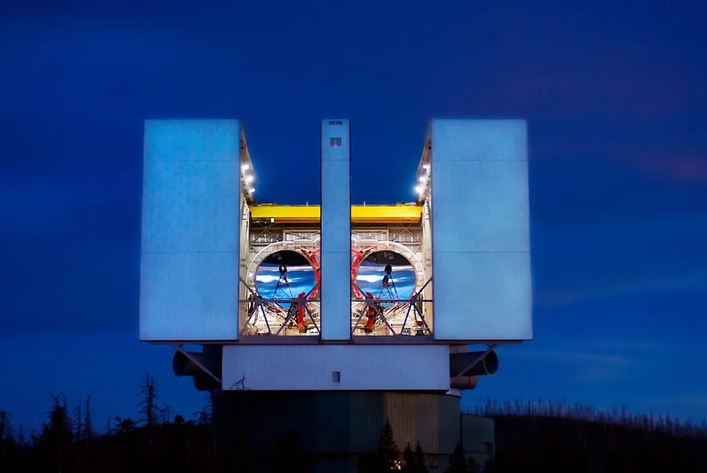
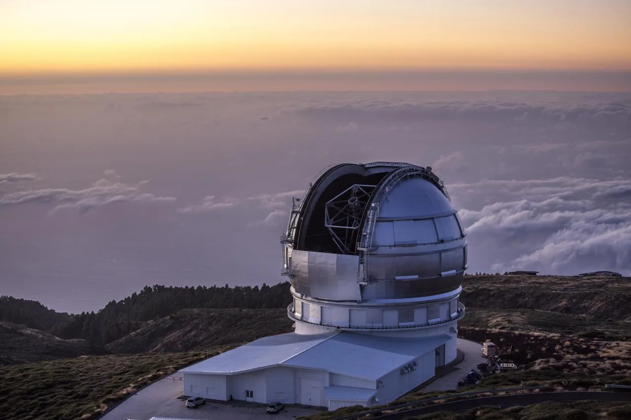
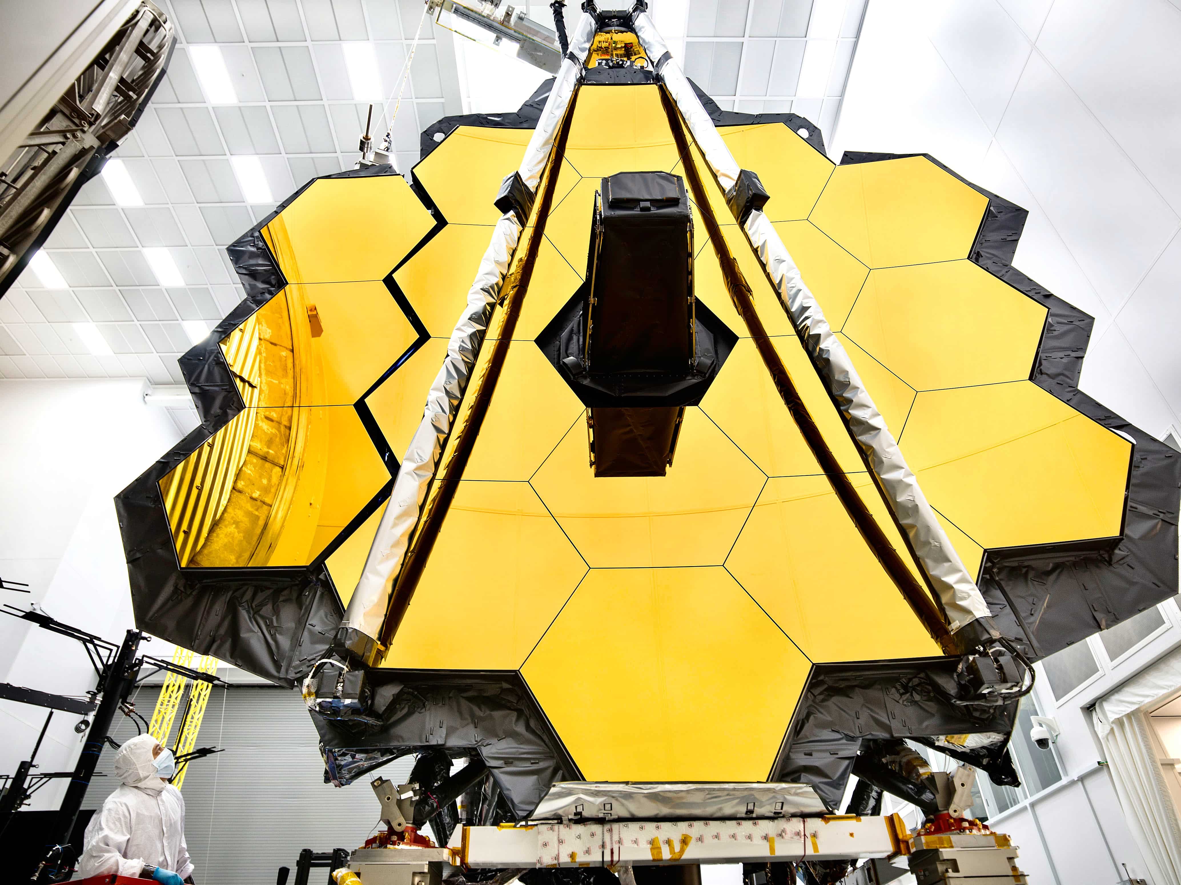
Now consider a telescope like Galileo's. If we wanted to build a bigger one we would have to manufacture a lens of large diameter, hence very heavy, difficult to mount on a structure and above all, stressed by its own weight, it would break, being fragile. If instead we use a mirror, we can rest it on a support that bears its weight when pointing at an astronomical object to be observed, and in this way much larger telescopes can be built with fewer problems. If you have already seen, in A bit of history, the discovery of infrared rays, you know William Herschel and his telescope of one metre in diameter, which could be built precisely because it had a mirror of that diameter. Currently the optical telescope with the largest diameter is the Large Binocular Telescope (LBT), with a diameter of 11.9 metres, though obtained by combining two mirrors of 8.4 metres each, while the largest single-mirror telescope ever built is the Gran Telescopio Canarias, 10.4 metres in diameter. Furthermore, the largest mirrors can now be built by mounting hexagonal elements side by side until large sizes are covered. One example is the James Webb Telescope, currently in space one and a half million kilometres from Earth. Below you can see some images of the telescopes we have listed.
Resolving power
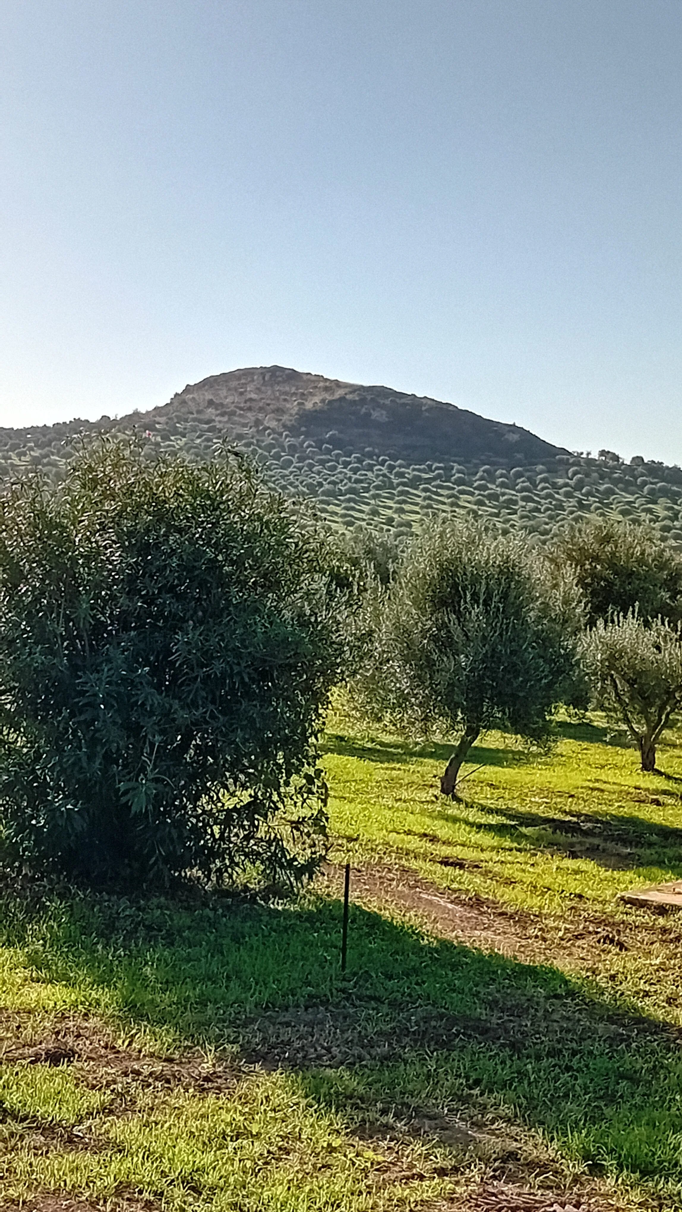
Another important quantity for a telescope is the smallest detail that can be observed. Look at fig. 6
In the foreground you can see two trees whose leaves you can make out clearly, but in the background there are other trees whose leaves cannot be distinguished individually. Intuitively, distance prevents us from seeing the individual leaves of the distant trees — but why? Let us see how resolving power works.
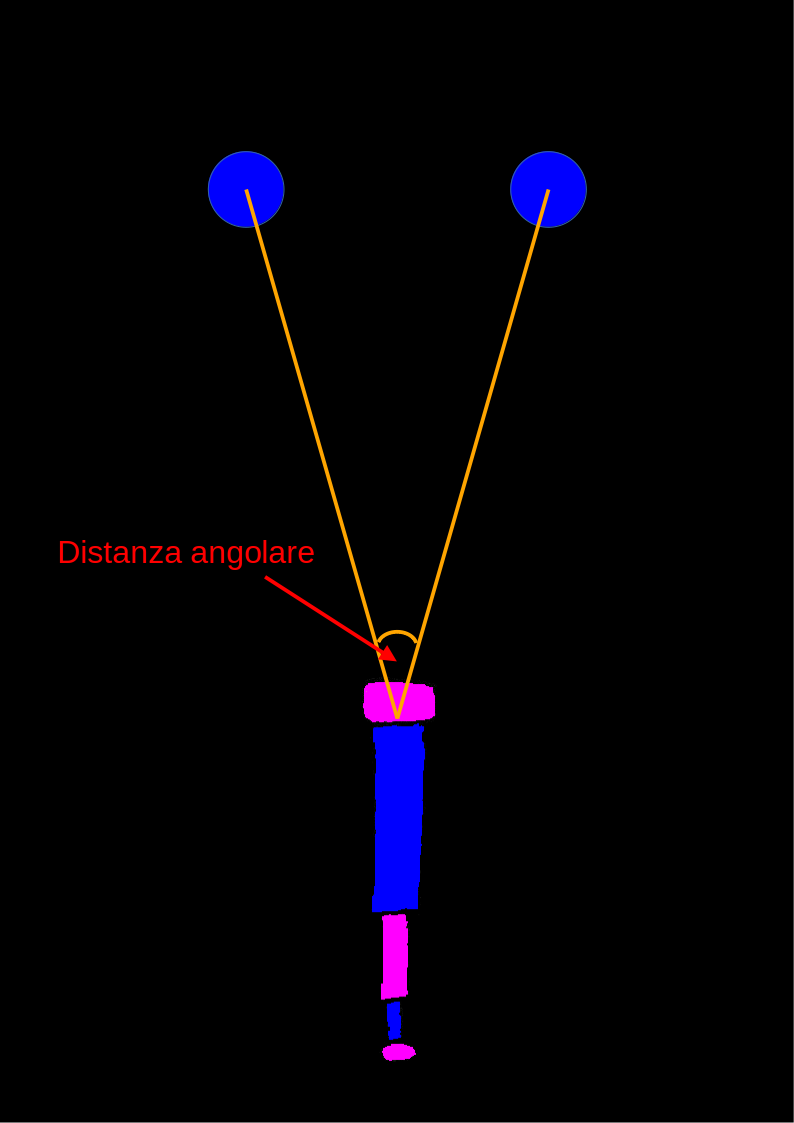
Consider the two blue dots in fig. 7 and their angular distance. The angular distance is obtained by imagining two rays leaving the telescope towards the two points, like the orange rays you see in the figure: the angle between these two rays is precisely the angular distance between the two points — the angle under which we see them.
Now consider the animation in fig. 8: the angular distance decreases as the telescope moves away from the two points. So the farther we are from the object we are observing, the smaller the angle between two details we want to distinguish.
There is a limiting angle, called the resolving power, which determines the smallest detail that can be distinguished from the others. If the angular distance under which we see two leaves is smaller than the resolving power of the eye, the leaves cannot be distinguished and will look like a single block. That is why the leaves of the nearby tree in the figure seen earlier can be made out, while those of the distant trees have much smaller angular distances between them, and the trees are seen as a single mass of green material.
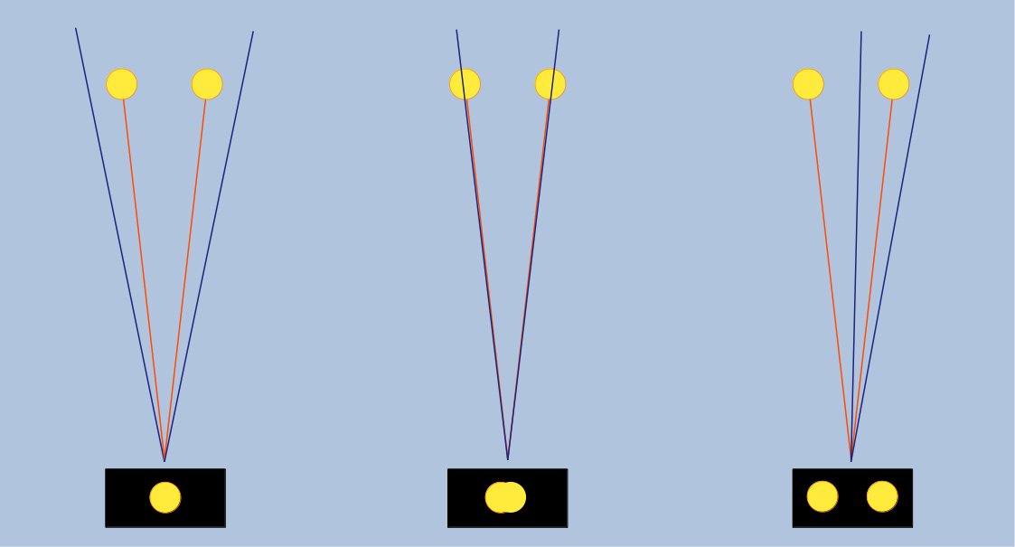
Let us see what happens in fig. 9. The angular distance (red lines) between the two stars is the same in all three examples, but the resolving power (blue lines) is different. Below each example is drawn what we would see with that resolving power and that angular distance. In case A the angular distance is smaller than the resolving power and we would see the two stars merged into a single source with the brightness of the two stars combined. In case B the angular distance is almost equal to the resolving power and the two stars are barely separated — they appear as an elongated object but are not yet fully distinct. In case C, finally, the two stars have an angular distance decidedly greater than the resolving power and are seen well separated from each other.
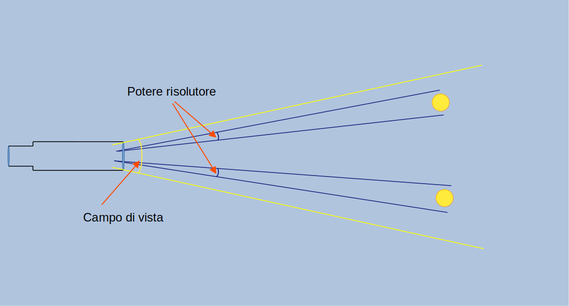
Be careful not to confuse resolving power with the field of view: the resolving power tells us the smallest "pixel" we can distinguish from the others, while the field of view is the whole region of space whose radiation manages to enter our optical instrument. An example is given in fig. 10.
The resolving power depends on two factors: the wavelength of the radiation at which we are observing and the diameter of the instrument we are using. In particular, the relation linking them is
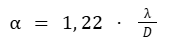
where α (alpha, a Greek letter) is the resolving power, i.e. the limiting angle in radians of our optical instrument, λ (lambda, also a Greek letter) is the wavelength, D the diameter of the instrument and 1.22 a proportionality factor.
This means that, given the diameter of an instrument and the wavelength of the radiation at which we are using it, we can know the minimum angular distance between details that we can distinguish. Let us take our eye as an example.
The wavelength of yellow light is 550 nm, nanometres (see also Electromagnetic radiation); the diameter of our pupil, in full daylight, can be taken as about 3 mm, so

that is, in arcseconds, α = 46”
Actually these numbers mean little unless one is familiar with angular sizes. Let us give some examples. The distance between a person's eyes is about 6 cm. Seen from afar, we would see the eyes as separate up to a distance of about 267 metres — that is, already at about 270–275 metres we would see the eyes on someone's face blurred into a single dark patch. Or, considering that the distance between the two headlights of a car is about 1.8 metres, we would begin to see them as a single light from a distance of about two and a half kilometres onwards. Or again, given that the leaves of a tree can be about 4 cm apart, we would see the crown as a single green patch, unable to distinguish the individual leaves, from 112 metres away.
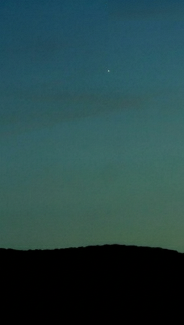
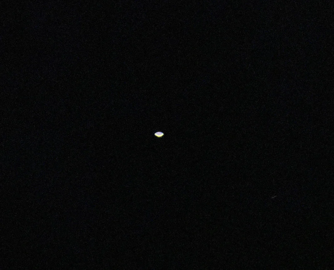
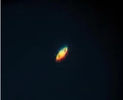
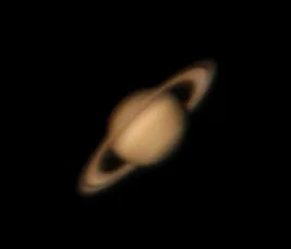
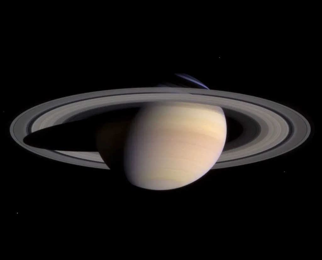
From the equation for the resolving power we see that the larger the diameter of the instrument, the better the resolving power, and hence the more details we can pick out. To appreciate this, look at fig. 11: it shows the planet Saturn as we would see it with the naked eye — essentially a bright dot. No detail of the great rings or of the banded structure is visible without a telescope. In fig. 12 we have instead three images obtained with telescopes of 5, 7 and 15 cm diameter respectively. Finally, in fig. 13 we see an image of Saturn taken by the Hubble Space Telescope, 2.4 m in diameter. The details increase as the diameter of the instrument grows, as we said, because the wavelength of the optical radiation at which we observe stays more or less the same.
The radio telescope
The radio telescope is, as its name says, a telescope for observing radio radiation. It is worth recalling, as already illustrated in the section A bit of history, that radio radiation was so named because it propagates in a straight line, along a "ray" — radius in Latin. Then, because of the use made of it, the device that for decades was the main medium of information also took its name, and we now call "radio" any long-distance audio communication system, apart from the telephone. Which, however, for about forty years now has itself been transmitting via radio — but let us not digress.
So, it is a telescope — from tele, a Greek prefix meaning far, and skopia, meaning to observe, to watch. A telescope is an instrument that observes from afar. Radio telescope means an instrument that does the same job as an optical telescope but observing radio photons. To find out what photons are and what we mean when we speak of the radio band, you can hop over to the section Electromagnetic radiation.
Structure of a radio telescope
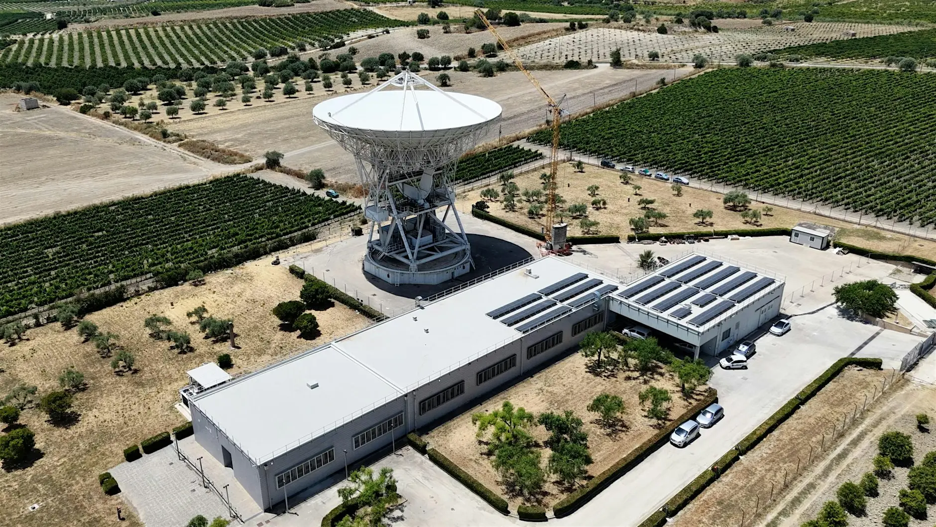
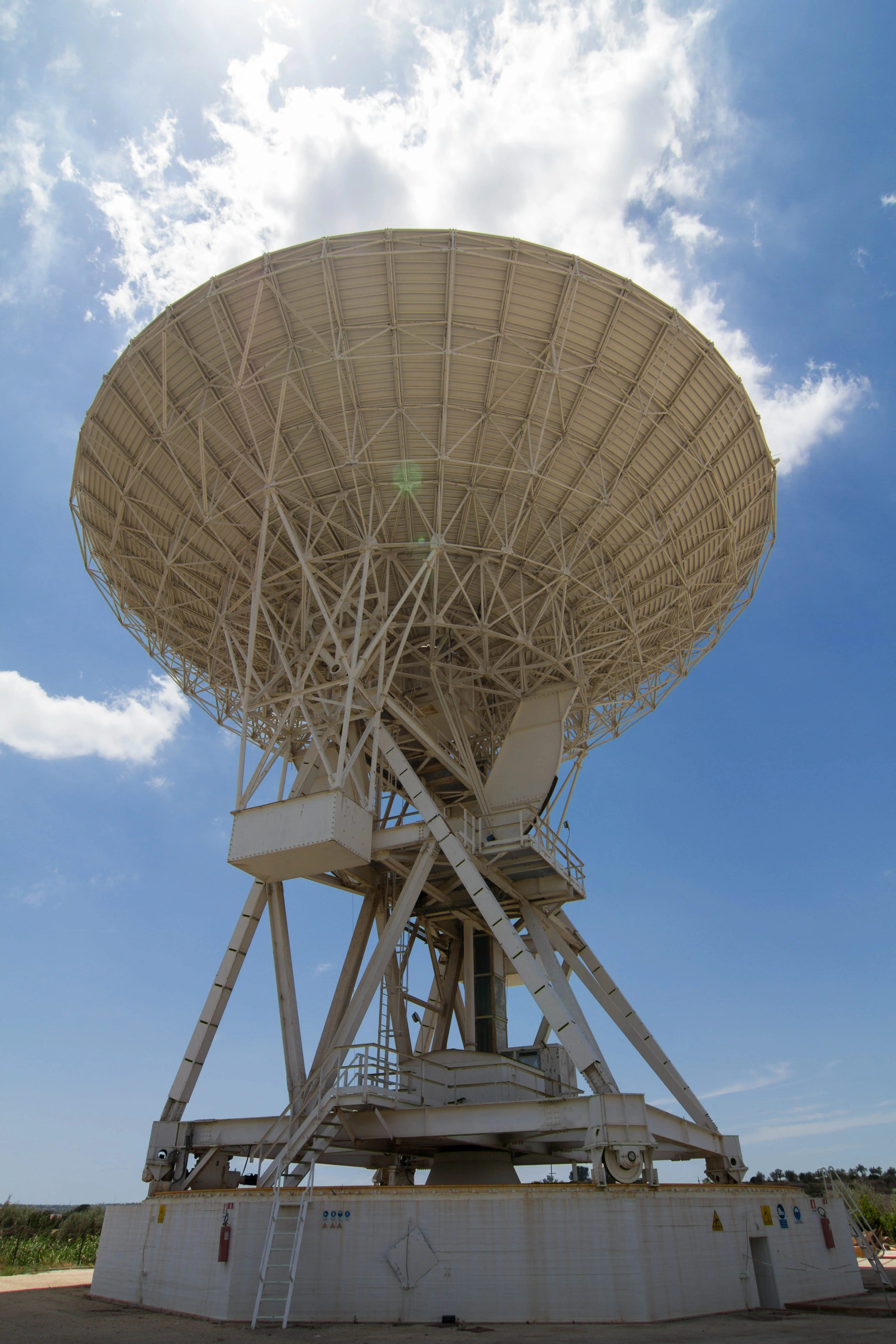
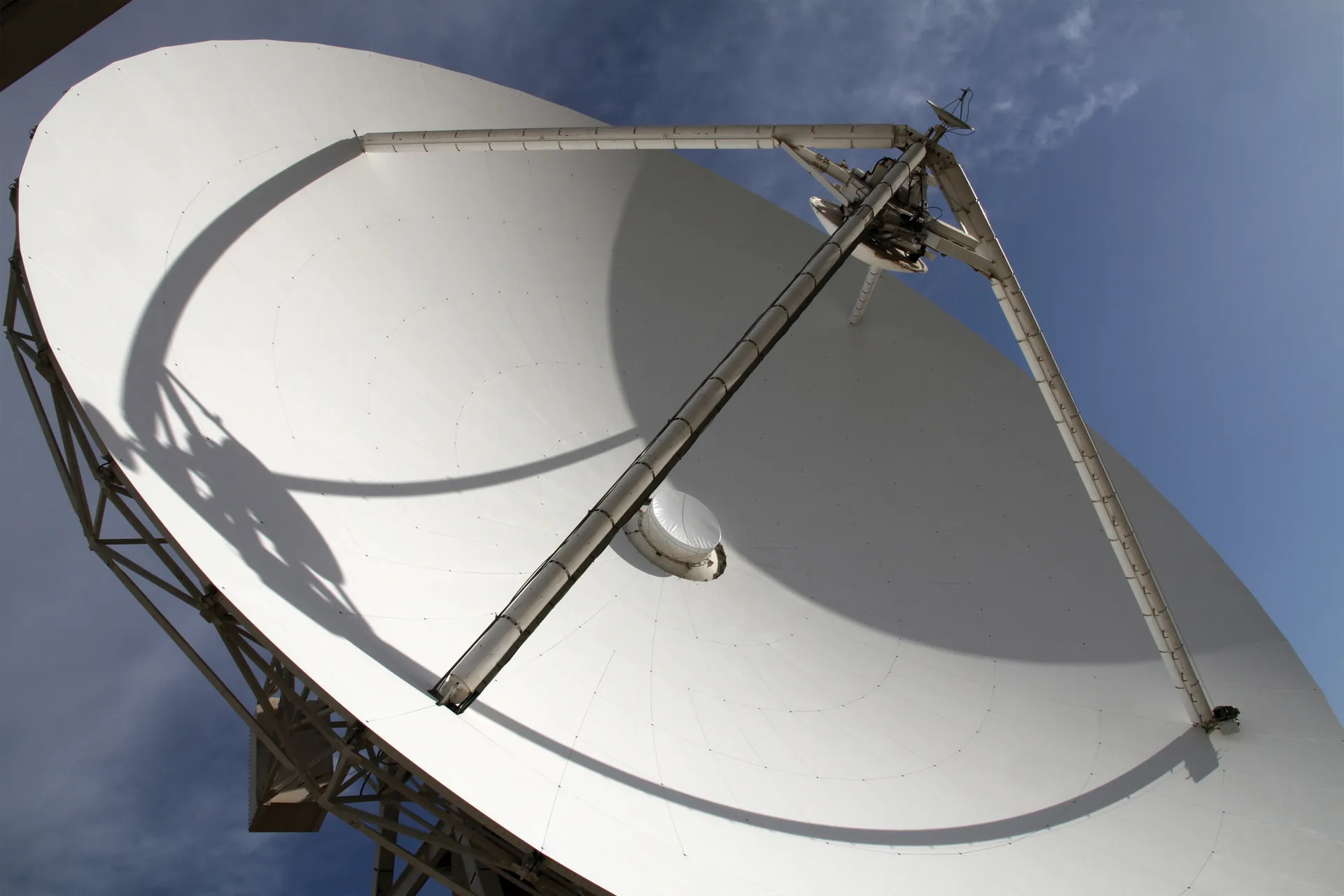
In fig. 14 we see two images of the Noto radio telescope. As you can see, it consists of a steel structure supporting the telescope proper. This structure rests on four wheels, two of which are driving wheels, rolling on a rail also made of steel. The rail is built to withstand the 310 tonnes of the complete radio telescope. Two stepper motors are mounted on two of the wheels and allow the radio telescope to be moved horizontally, letting it point in any direction through 360 degrees. The structure holds a basket made of steel girders which in turn supports the primary mirror — the white panels you see in the second image. The basket is mounted on a horizontal axis, and two motors raise and lower it to steer the primary mirror up and down. In this way, moving the antenna horizontally and vertically, we can point it precisely in any direction of the sky, to observe specific sources whose position we know.
Let us start by noting that I told you the white panels, made of aluminium and painted with materials inert to electromagnetic waves, constitute the primary mirror. Of course you have a very different idea of a "mirror": in a mirror you see the images of your surroundings reflected, not barely the light that illuminates it. I must contradict you: for electromagnetic radiation, a mirror is any surface whose imperfections are smaller than 1/8 of the wavelength of the radiation itself. This means that any surface with this characteristic reflects electromagnetic radiation.
But then why can't we see ourselves reflected in this strange "mirror" of such an imposing diameter? It all depends on the wavelength of the radiation involved. Your mirror at home, to do its job, must reflect radiation with a wavelength of, say, 550 nm (nanometres), so it must have imperfections smaller than about 68 nm. Picture a millimetre on any set square: the imperfections of your mirror must be almost 15,000 times smaller than that millimetre! Only then can you shave or put on make-up while seeing what you are doing. But what if the radiation were radio? A typical wavelength in the radio band is 21 cm. So an imperfection on a surface that is to reflect radiation of that wavelength without compromising it must be smaller than 2.6 cm. Look at your hand with the fingers spread, or if you like imagine a net with meshes less than two and a half centimetres apart: these are mirrors for radio radiation at 21 cm.
That is why the primary mirror of our radio telescope needs no polishing like optical telescopes do.
The motors that move the antenna also have the task of moving it extremely slowly, imperceptibly to the eye. This is because, after pointing the radio telescope at a source, we may need to observe it for very long times, from a few minutes to several hours. And what about the Earth's motion? We see the Sun move across the sky because it is the Earth that rotates on its axis, making the sky above us appear to be in continuous motion. Sources in the sky move just as the Sun does, and if we must keep the antenna pointed at a source for a long time we must "track" it — compensate for the apparent motion of the source in the sky by moving, in turn, the telescope or radio telescope observing it. But for the same reason that watching the Sun gives us no sense that it is moving — its daily displacement is extremely slow — tracking a source likewise requires moving the antenna slowly but precisely, to keep it pointed at the source under study at all times. These motors are therefore powerful yet extremely precise, and can genuinely move the antenna by millimetres.
Our telescope, too, has a mount like those illustrated earlier — indeed, it has both. In fig. 15 we see an optical diagram of the Noto radio telescope.
The primary mirror is the blue curve, and the radiation arriving from space is represented by the orange traces. After reflecting off the concave primary mirror, the radiation heads towards the focus, where the receiver sits. In this case the radio telescope is arranged in the Newtonian configuration. As can be seen in the animation, the radiation reflected off the primary mirror is gathered by the receiver from the whole mirror, all at once.
Now let us look at the animation in fig. 16
In this case, in place of the receiver there is another mirror that reflects the radiation again towards another focus, located behind the primary mirror. If you compare fig. 16 with fig. 5 you will realise that this is a Cassegrain mount, with a concave primary mirror and a convex secondary. In this way we can place some receivers at the Newtonian focus, letting the radiation reach them by mechanically moving the secondary mirror aside, and others at the Cassegrain focus, which the radiation reaches when the convex mirror is put in position, covering the receivers at the Newtonian focus.
At the focus, be it Newtonian or Cassegrain, the receiver is arranged as described in the section The acquisition chain of a radio telescope. The first component the radiation meets as soon as it is reflected by the mirrors is the horn, an instrument shaped like a truncated cone that funnels the radiation towards the truly sensitive part of the receiver. Its shape stems from the need to receive all the radiation coming from the mirrors or, as the jargon goes, to illuminate the mirrors. Let us look at fig. 17
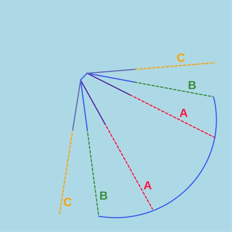
There are three examples of how the horn of a receiver might be shaped. In case A the horn is too narrow and the radiation coming from the outer parts of the mirror does not enter it, and is thus lost. In case C, on the contrary, the horn is too wide open, letting into the receiver radiation that does not come from the mirror, increasing the noise and distorting the measurements of the radio telescope. In case B the horn has exactly the right opening to illuminate the whole mirror and nothing more, without losing signal or introducing spurious signal. We use the term "illuminate" because of what we call the antenna reciprocity theorem: an antenna can be used both to receive and to send radio signals, so an antenna behaves in the same way in reception as in transmission. Illuminating the mirror means that, if we wanted to send a signal from our radio telescope, we could do so using the same horn used for reception, thereby illuminating the mirror with the transmitted signal.
Like any other telescope, a radio telescope also needs a large diameter to ensure sensitivity and resolving power. But for radio radiation the resolving power is decidedly critical. Let us try to calculate the resolving power for radiation with a wavelength in the radio domain (see Electromagnetic radiation) — say 21 cm — observed with a radio telescope 1 m in diameter

that is, α = 14.7°
Do you know what the smallest detail it could distinguish would be? An object as large as 28 full Moons! Practically speaking, a three-storey house seen from fifty metres away would appear as a single grey block of roughly roundish shape. Very large instruments are therefore needed to distinguish the Moon from another object not far from it. Our radio telescope is 32 metres in diameter. Let us see its resolving power at 21 cm

that is, about 28’ — the angular size of the Moon. This is why radio telescopes must be at least as large as ours: only in this way can we distinguish objects in the sky from one another; otherwise, nearby objects would be blurred together like the two stars of case A in fig. 6. To understand how images are degraded, let us look at fig. 18.
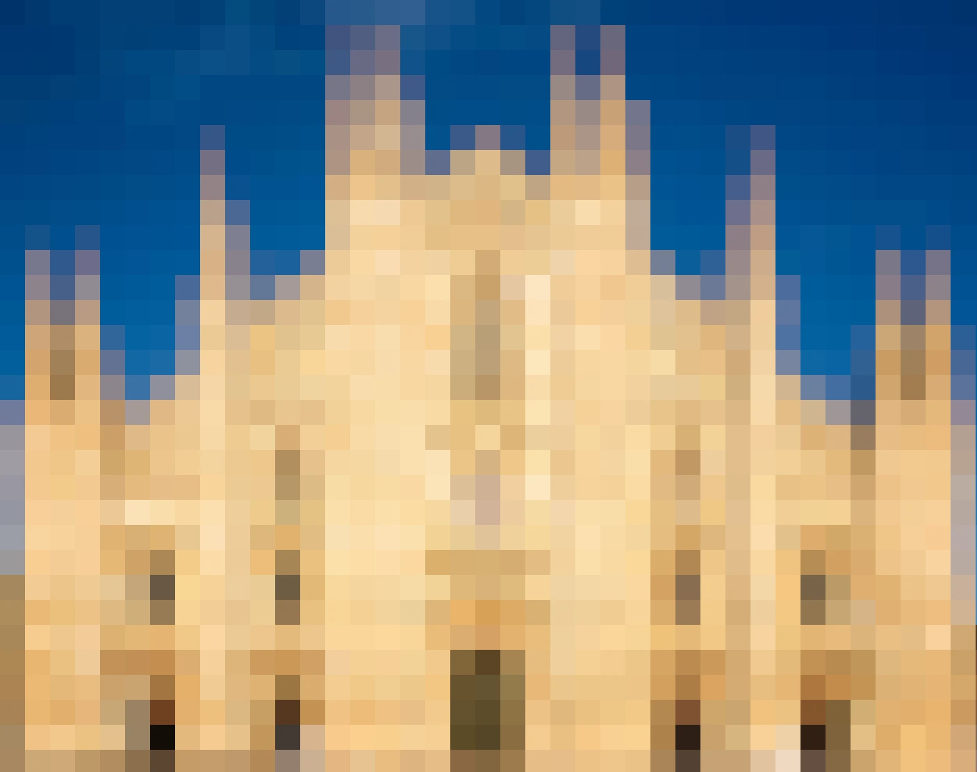
There is no need to tell you that this is the Milan Cathedral as we would see it with our own eyes. We said that our eye has, in yellow light, a resolving power of 46’’, and that this power lets us see all the details of the Gothic façade you see in the photo. But what would happen if it were our Noto antenna looking at the cathedral at a wavelength of 21 cm? Of course, we assume the cathedral is visible at that wavelength — but if we were to "take a picture" of it (we will see further on that it is not so simple in the radio band) we would see what appears in fig. 19
Most of the details are no longer visible, blurred into large pixels — so large as to merge the details into a single bright spot whose colour is the blend of all the colours present in that area. Let us try increasing the diameter and send the Effelsberg radio telescope, near Bonn in Germany, to the cathedral square. Its diameter is 100 m, so its resolving power is more than three times better than that of the Noto radio telescope. What it would see is in fig. 20


Yes, a few more details, but nothing comparable to our eyes. If we wanted to obtain a picture in the radio band with the resolution of our eyes we would have to build a radio telescope 942 metres in diameter!
Another important role of the resolving power is distinguishing two sources from each other, as seen in fig. 6. It is the ability to tell two objects apart instead of seeing them "blurred" into a single cluster of pixels in the image. To explain it, let us look at fig. 21
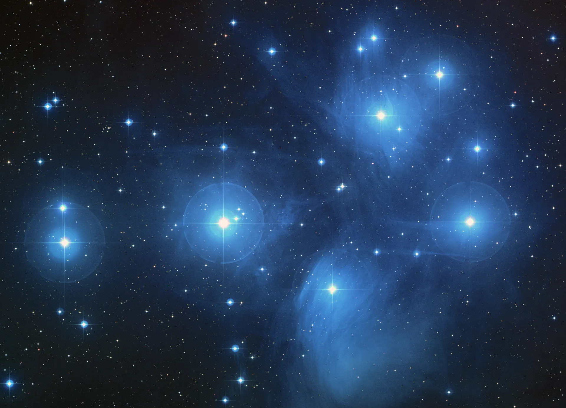
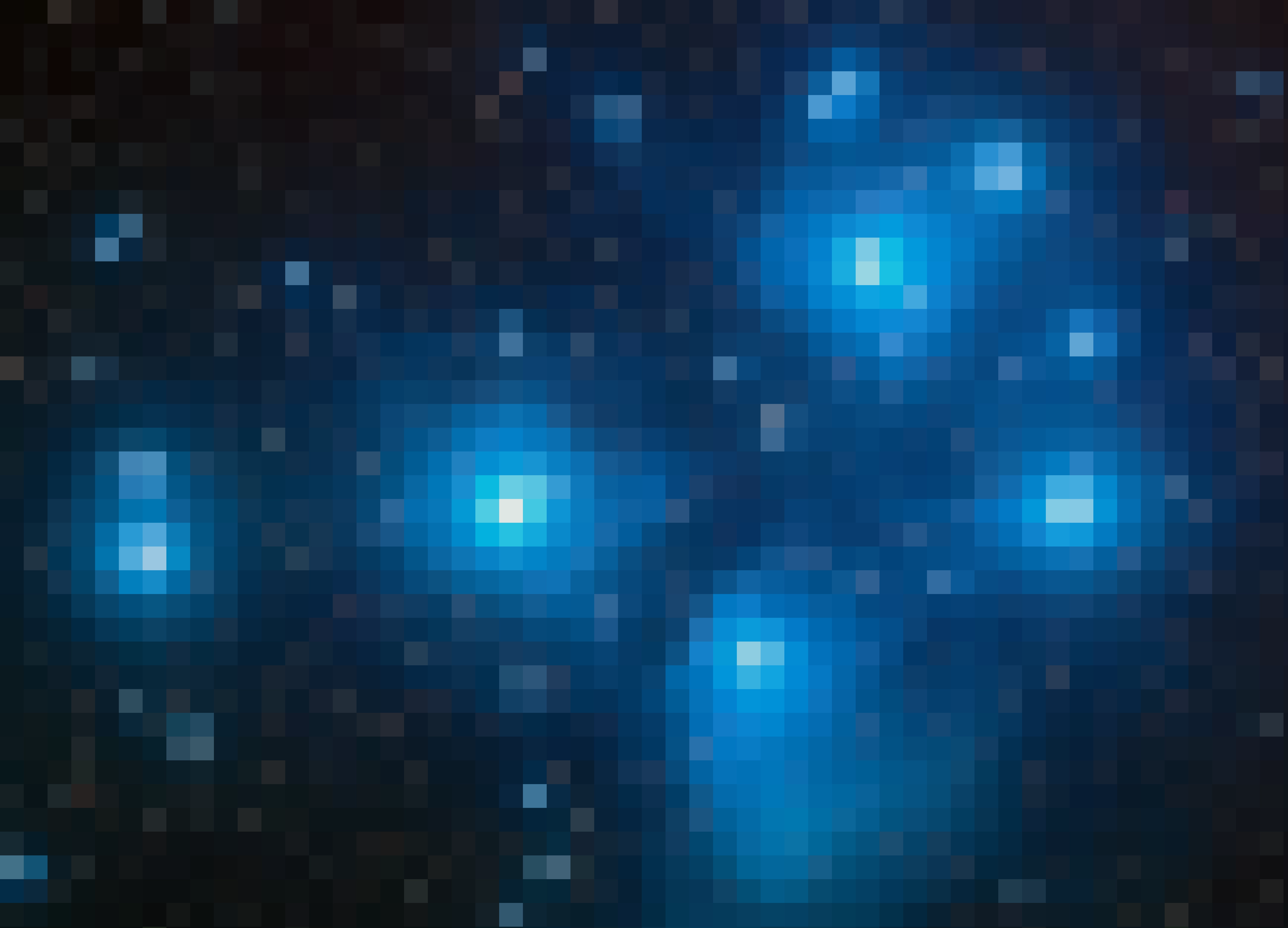
Here we see the Pleiades, an open star cluster visible in the constellation of Taurus, next to the brightest star of the constellation. The seven stars visible even to the naked eye were identified by the Greeks with the seven sisters, daughters of the titan Atlas and the nymph Pleione. The photo was obtained with a resolution high enough to allow even the faintest stars of the cluster to be distinguished. Now let us artificially reduce the resolution of the photo.
In fig. 22 we see that the brightest stars are still distinguishable, though not as clearly, while the smaller, fainter stars cannot be told apart from others very close to them. The better the resolving power, the better we can distinguish the individual sources.
The resolution problem in radio astronomy
We have seen that resolving power is decisive for observing the details of a source, or for distinguishing one source from another when they are points of light. But we have also seen that the resolving power of a radio telescope is decidedly worse even than that of the human eye — let alone the resolution of a good telescope, or of the most powerful ones. It would seem that observation in the radio band must suffer from a structural weakness: the impossibility of seeing details useful for studying the sources that emit in the radio band. And yet in 1967 radio astronomers got the better of this, using a system that is elaborate, complex, impossible to implement without computers, but decidedly effective in improving the resolution of radio images: interferometry.
You should know that when electromagnetic radiation passes through an aperture — be it a hole, the mouth of a telescope or even a concave mirror, in short anything with boundaries — it undergoes an important modification which we have been able to model with a mathematical function. Put simply, if we consider a wave in general, and an electromagnetic wave in particular, we can describe it with a mathematical function before and after it has passed through the aperture we mentioned. There is a mathematical function relating the two moments, which we call the Fourier Transform, after the French mathematician who developed it. If, before reflecting off the concave mirror, the electromagnetic wave can be represented by a certain function, after the reflection the wave is represented by the Fourier transform of that same function. And the process is reversible. We can see it with an example. If you put your right hand in front of a mirror, it will look like a left hand: if you look at your left hand with the palm turned towards you, you will notice it is identical to the reflection of your right hand seen in the mirror. But if we reverse the process and consider the reflection of your left hand, it will appear as a right hand. The mathematical "function" in this case is the reflection of the mirror. If what is reflected is a hand with the thumb on your left (that is, a right hand — try it!), in the mirror you will see a hand with the thumb pointing right, like your left hand, obviously when seen palm-side. And, of course, vice versa. Mathematically this can be represented as the inversion of the x-axis of a Cartesian coordinate system. Shall we complicate the experiment? Take a spoon or, better still, a metal ladle. Put the index finger of one hand in front of the ladle, on the concave side: you will notice that the reflected image is flipped, upside down with respect to how you held your finger. Now flip your finger: you will see the reflection flip again and remain upside down with respect to your finger. The electromagnetic wave we call light (see Electromagnetic radiation) reflects off your finger, bounces again off the ladle and reaches your eyes. Before the reflection the light has one direction; after the reflection its direction is changed. As with everything, we can represent this change with a mathematical relation, which in our case is the Fourier transform. This is definitely not the place to explain what it is, but suffice it to know that applying this function to the image transforms it into the object, and vice versa. So, when observing an object in the sky, by collecting its image in whatever way, we have its Fourier transform, and by applying the inverse Fourier transform to the image we get back the object as it appears in the sky.
This is what radio interferometry is based on. Instead of observing with a single radio telescope, we collect the image of an astronomical object with a system of many radio telescopes scattered over a region. They can be tens, hundreds, even thousands of kilometres apart or more. When we observe these objects, we record the signal on SSD storage and later combine all the observations made by each single radio telescope with those of all the others that took part in the observation. This operation, too, is done with mathematics — an operation called correlation. Once this has been done for all the collected data, we have a set of correlated data, all in a single file. At this point we apply the Fourier transform to this data set and voilà! We transform these data back into an image as it appears in the sky. This time, however, the resolving power no longer depends on the diameter of the single antenna but on the distance between the antennas. In short, this operation has improved the resolution thousands of times, in proportion to how far apart the radio telescopes that observed were. An example? If two radio telescopes are 50 km apart, the resolving power along the direction joining them will be

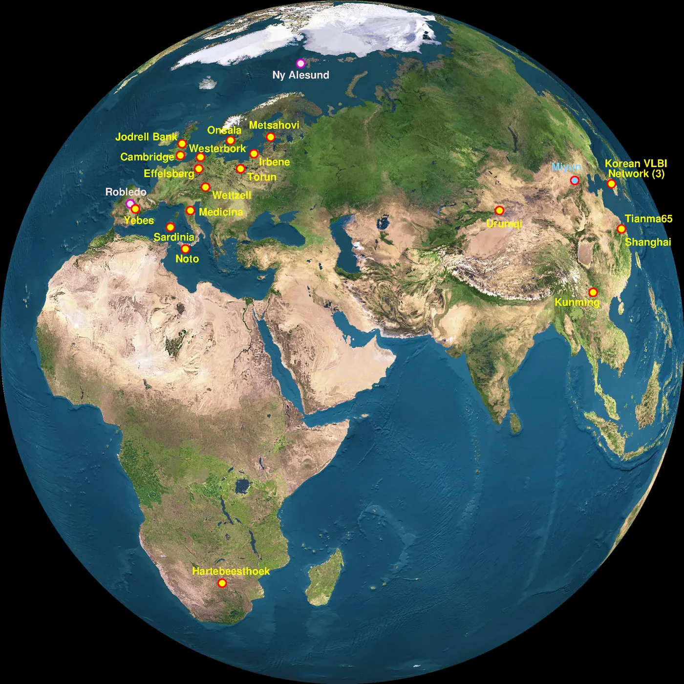
that is, α = 1´´ — similar to the best ground-based optical telescopes. But we can do better. In fig. 23 we see the European VLBI Network, where VLBI is the acronym identifying the radio interferometry technique used, called Very Long Baseline Interferometry — where the very long baseline is the distance between the antennas involved, which can be as much as about ten thousand kilometres.
The EVN is made up of 19 radio telescopes, built at different times, which have been carrying out joint observations for more than forty years now. The resolution achievable with a baseline about ten thousand kilometres long is, at the usual wavelength of 21 cm

that is, five thousandths of an arcsecond. Going back to the photo of fig. 9, we could see the leaves of a tree as clearly distinct from a distance of 1600 kilometres!
How do you take a picture in the radio band?
And back to the initial question: can we take a "picture" of an astronomical object in the radio band? Yes, we can — under certain conditions.
Let us start by considering making an image of an object with a single radio telescope. As we have seen, the resolution of a telescope on its own does not let us do much, but there are objects whose angular size is much larger than the resolving power of a single radio telescope. In this case we run into another obstacle: the radio telescope "sees" only one pixel at a time! We can see it here, in fig. 24
In this image we have drawn a mirror like that of a radio telescope, but the object being observed is extended.
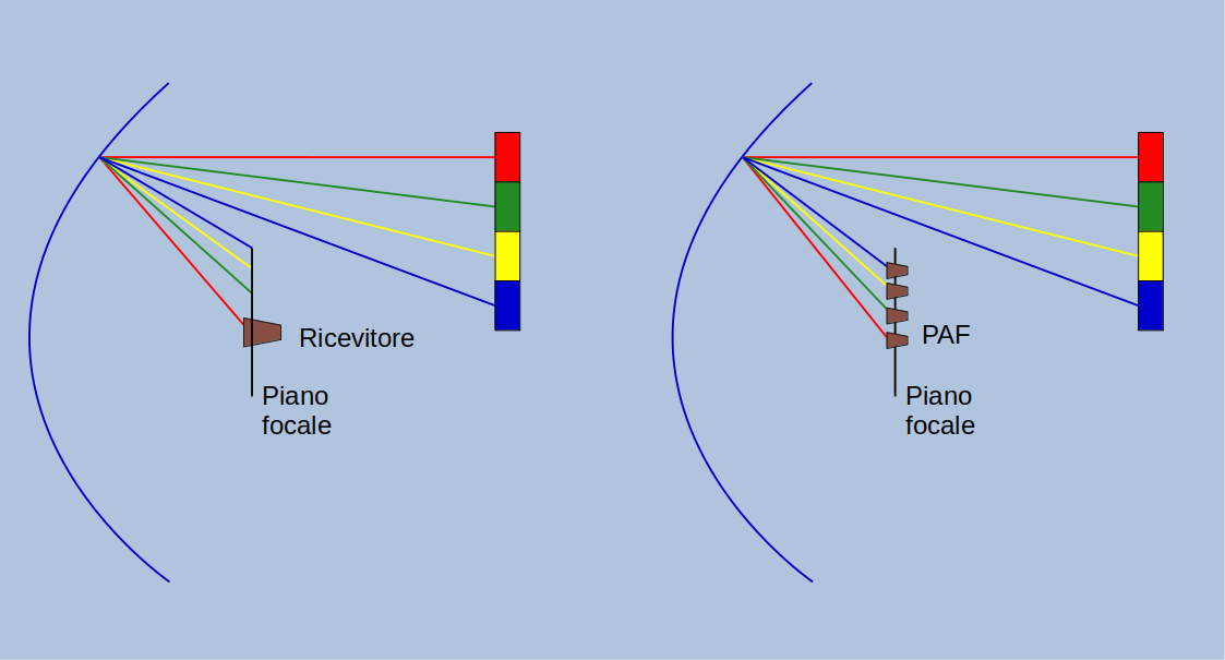
From every point of the object a light ray arrives and is reflected onto a different point of the focal plane, a plane passing through the focus on which the image of the object forms. In the case of the radio telescope, the receiver sits only at the focus and there is nothing else on the focal plane to collect the radiation. It is as if a camera had only one pixel, at the centre: in the figure, only the point coloured red will be visible to the radio telescope. The other points will be visible only if the radio telescope is pointed in a different direction.
There are systems for obtaining a sort of focal plane for radio telescopes too, and a diagram of what they look like is shown on the right-hand side of the figure. They are called Phased Array Feeds (PAF) and are receivers with a grid of sensitive elements side by side, which make it possible to detect the radiation coming from many points of the observed object simultaneously and without moving the radio telescope. This is one of the systems that can be used to create an image of a region of sky, provided the object we want to image has an angular size larger than the resolution of the antenna at that frequency. But PAFs are instruments used on a small number of radio telescopes, such as the Australian Square Kilometre Array Pathfinder (ASKAP) or the Effelsberg radio telescope in Germany, and only for a limited range of wavelengths. The Noto radio telescope is not equipped with these receivers, so we must resort to another solution.
Since, as we have seen, the Noto antenna can see one pixel at a time, we can reconstruct an image by taking the image of the individual pixels. Look at fig. 25.
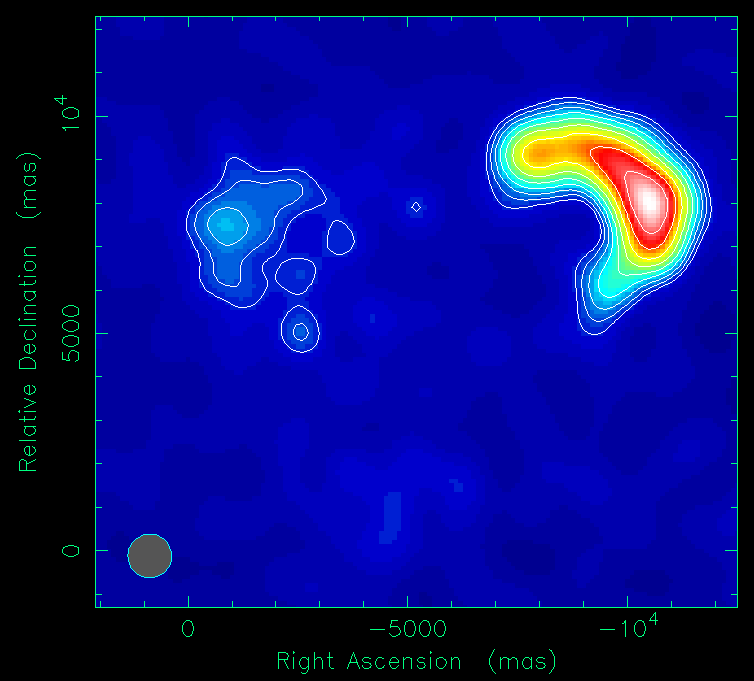
The blue frame you see is a region of sky of which we want to make a radio image. At the bottom, the antenna points, one at a time, at a square of sky the size of the resolving power. The radio telescope points at an area, acquires its brightness through one of the back-ends and the data point is recorded. The collected data can then be used to represent the radio image of that region of sky through an isophote diagram. Let us watch the animation in fig. 26
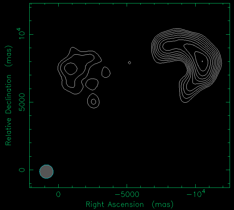
The region of sky is observed one "pixel" at a time — the antenna points in one direction within the frame we want to image and acquires the radiation coming from that point. A number is recorded corresponding to the radio brightness perceived by the antenna. Suppose there are points where the antenna "reads" a brightness value of 1. All those points are marked with that value on the diagram of fig. 28. Other points will have a value of 2, and those too are marked with their value. Finally, the points with a radio brightness value of 3 are marked. Now let us join the dots, as in puzzle magazines — but this time, instead of joining them in numerical sequence, we join the dots with the same value. You can see that closed lines form along which all the points have the same brightness: these lines are called isophotes, from the Greek "isos", equal, and "photos", light. They are lines along which the brightness is the same at every point. In this way we can draw closed lines enclosing areas where the brightness is greater than outside them. If inside the first line we draw the isophote with the higher brightness, we get a second curve which in turn encloses an area brighter than both the region between the two lines and, of course, the rest of the frame. The third isophote encloses an area of still greater brightness, and so on until the maximum brightness in the whole frame is reached. In this case we will have a radio source with an elongated shape and a brighter central region fading towards the outside. In fig. 27 we can see some radio images obtained with this same isophote visualisation system.
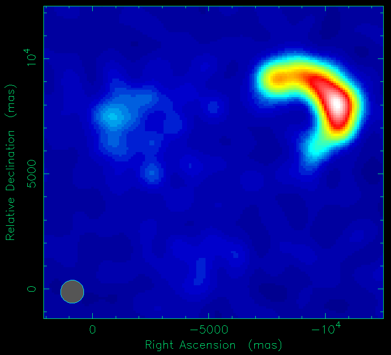
As you can see, each source has its own peculiar shape and brightness, which will allow us to study its structure and the phenomena that generate its radio emission. The same images can also be rendered in "false colours", as you see in fig. 28.
Here the areas between the isophotes are coloured with colours that do not really exist, since radio electromagnetic waves have no colours. A false-colour reconstruction better highlights the different regions of a radio source to the human eye, which is much more sensitive to differences in colour than to differences in brightness.
The technique we have illustrated — observing point by point with an antenna — is called nodding, but it is not the only system. We can also obtain maps by scanning, a system in which the antenna sweeps continuously across the region to be observed while never ceasing to take data. It is a faster system but sometimes less sensitive.
Finally, the VLBI technique we saw earlier also makes it possible to obtain images like those shown. This is because the data collected by the various antennas and correlated is then processed with the Fourier transform. This operation is carried out in a discrete way — on a grid of pixels, point by point — where the size of the individual pixels depends, as we have seen, on the maximum distance between the antennas involved in the observation. By mapping the illumination of each point onto a grid on the screen and producing an isophote or false-colour diagram, we obtain images similar to those obtained by mapping, but this time of objects whose total size is enormously smaller than what can be achieved with nodding or scanning.
What we do with these images is described in the section Observing in the radio band
Brightness measurements
One of the oldest measurements of astronomical objects ever made by humankind is brightness. When we possessed no instrument capable of magnifying the sources in the sky, one could still notice that some stars were brighter than others. Comparison by naked eye is not very accurate, but it was used for so long that the system of magnitudes for measuring the apparent and absolute brightness of astronomical sources is still in force today. In any case, in the radio band as in all the others, brightness measurements can be made, using techniques somewhat different from those used, for example, with visible light. Let us see how a radio flux — and hence brightness — measurement is made.
First let us define the flux of a source as the amount of energy we receive per second and per square metre. In the radio band, in particular, we use a unit of flux per unit frequency. We call it the Jansky, after Karl Guthe Jansky, an American physicist of Czech origin who was the first to observe — by chance — an astronomical source in the domain of radio waves. The value of one Jansky is
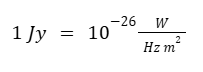
Just to grasp how small this unit is — and thus how faint the sources we observe are — at the frequency of 1 GHz, i.e. one billion Hertz, the Sun has a radio flux of
106 – 108 Jy, i.e. 10-18 W Hz-1 m-2, and it is right around the corner; yet many sources have a flux of 1 Jy or even much less. We know of sources of 50 millionths of a Jy.
Think how sensitive our radio telescopes are!
Now we must consider how to derive the correct flux from the recorded data. In fact, as can be seen in the section The acquisition chain of a radio telescope, what we record is a current, which we must relate to the energy of the photons that arrived from the source under examination. In optical astronomy this is achieved simply by comparing with a source of known flux, since there are plenty of them in the sky. But radio sources are not only far fewer in number: many are also variable, and therefore unsuitable to be used as reference sources or calibrators. In this case we exploit the possibility of producing an artificial radio signal through a calibrated diode, comparing the energy collected from the source with the calibrating diode, which we call the noise diode (or noise cal).
Finally, we measure the flux of the source by comparing it with the flux of the sky in its surroundings, which must be empty of other sources. This operation can be done in two ways.
The first is called on-off. As the name itself says, we point the antenna at the source (on) and take a measurement, and then repeat the same measurement pointing the antenna off the source (off). The difference in the recorded signal is the signal produced by the source, and comparing this signal with the noise cal gives us the flux of the source in Jy. The operation is carried out several times, taking the antenna off-source in different directions — typically the four positions above, below, right and left of the source, drawing a cross around it. (fig. 29)
The second method is more precise thanks to the speed of measurement and is called the cross scan. The antenna is taken off-source by a certain angle and then swept across the source until it passes beyond it by the same angle on the other side. Watch the animation in fig. 30.
At regular, very small intervals (about 30 measurements per second) a measurement of the energy received by the antenna is taken. With these data it is possible to reconstruct a plot like the white trace in fig. 30. The central peak you see is precisely the source we are examining, and its maximum is the flux we were looking for. This too is calibrated with the noise cal to obtain the value in Jy, and in this case as well we make several measurements in a cross pattern, doing one scan in azimuth and one in elevation — hence the name cross scan (see The radio telescope).
And the luminosity? What we have found so far is the flux of the source, i.e. its apparent brightness, given by the combination of the power of the source itself and its distance. To obtain the luminosity we need the distance, which can be obtained with different methods depending on its magnitude. For galaxies, for example, we use Hubble's law, which establishes how the redshift of a galaxy's spectrum is correlated with its distance. Once the distance is known, the luminosity is obtained simply from the relation
L = F · 4πD2
where L is the luminosity, F the flux in Jy, D the distance of the galaxy in question, and π we all know.
Measuring the luminosity of a source is useful for relating this luminosity to other characteristics of the source, to understand whether there are links between the various phenomena taking place in it. Moreover, the variability of the source, obtained through flux measurements made at different times, can give important information about the size of the emitting region and the physical mechanisms at work.
Radians
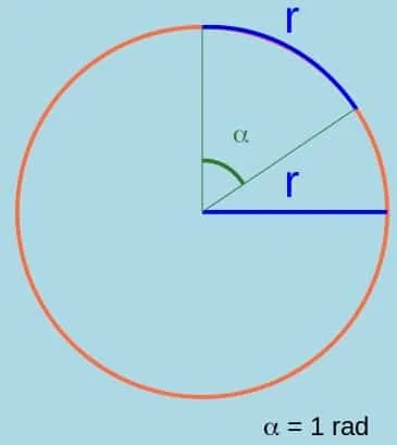
A radian is a unit of angular measurement based on the ratio between a circumference and its radius (radian comes from radius, Latin for ray). A radian is the angle that would be marked out if we laid the radius of a circle along its circumference, as shown in the figure.
CCD
CCD stands for Charge Coupled Device. These are instruments in which a layer of semiconductor material is made more sensitive to the photoelectric effect, an effect that allows the electrons of a material to be torn from their atom and either escape the material or move freely within it. Under the action of light on a point, roughly as many electrons are freed as photons arrive at that point, and the charge remains trapped by an electric field that captures the electrons. By counting the electrons of each point, which we call a pixel, one can know how many photons have arrived, and from the number of photons arriving on all the pixels a two-dimensional image can be reconstructed.