
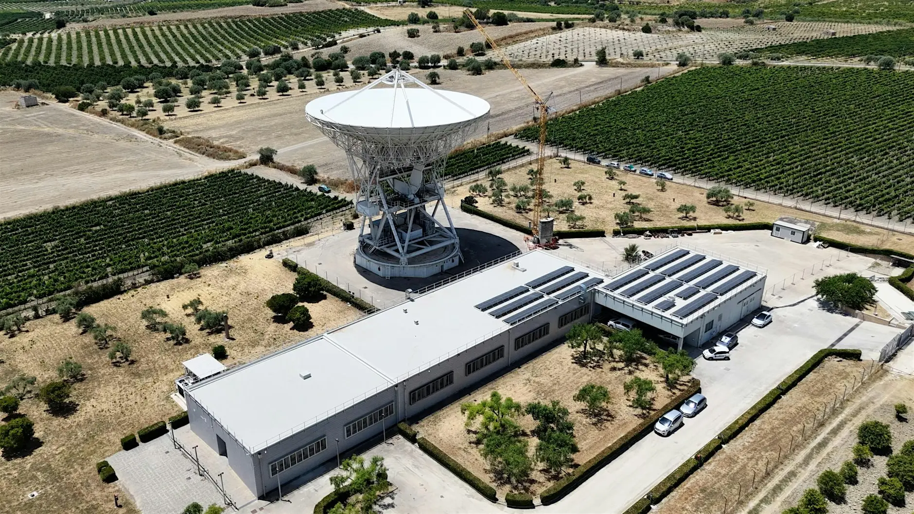
A radio telescope like the one in Noto is designed to receive low-frequency electromagnetic waves known as radio waves. This type of radiation is emitted by a variety of astronomical objects (active stars, radio galaxies, quasars: a more detailed list of astronomical objects that emit in the radio band can be found in Observing in the radio band) which can be studied to understand the mechanisms behind them.
Receiving and recording — in one word, acquiring — radio waves is done through a rather complex system that we call the acquisition chain. It is a series of instruments used to collect, amplify, split and record the signal coming from an astronomical object.
The first element of the chain is called the front-end: it is the part that is sensitive to radio waves, the instrumentation that turns the signal received in the form of photons into an electrical signal that can be amplified and read by other instruments. Then, through a system of converters that transform the analogue electrical signal into an optical one, the signal is transferred to the second stage, the IF distributor, after being converted back to analogue at the end of the optical fibre. From the distributor the signal is sent to the various back-ends, some of which are permanently installed at the Noto Radio Astronomy Station, while others will be in the future, or can be installed at the Station by the researchers who developed them because they require a particular type of observation.
Finally, the data are recorded by the recorder, which also depends on the type of data to be recorded and on the back-end being used.
Front-end
Radio electromagnetic radiation (see Electromagnetic radiation and Radio waves for details) emitted by an astronomical object travels for times ranging from a few minutes up to several billion years, and when it arrives here, the front-end is the first element of the acquisition chain it encounters. The first instrument that "sees" a radio photon is the horn, a metal structure built in a particular way, as in figs. 1a and 1b
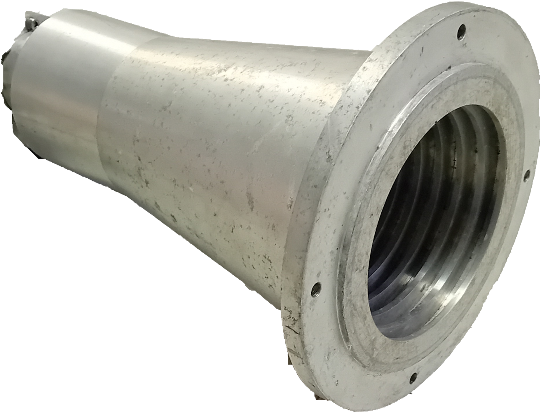
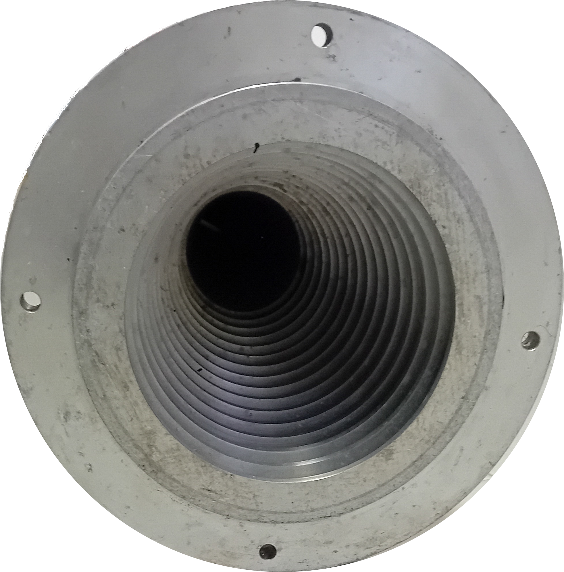
A horn is generally made of aluminium, a conducting material, because it has to "interact" with the electromagnetic wave. A structure that allows the electromagnetic wave to propagate inside it with minimal losses is called a waveguide. In fig. 2 you can see the cross-section of a horn. The conical shape and the corrugation — the "fins" you see in the figure — are there to offer the least possible resistance to the propagation of the wave along the horn, so that the radiation can be guided with the smallest possible loss down to the truly sensitive part of the front-end. They are closely related to the wavelength (λ) of the received radiation: the depth of the corrugation must be around ¼ of the wavelength of the radiation to be collected, and the spacing between the fins must be about ⅓ λ.
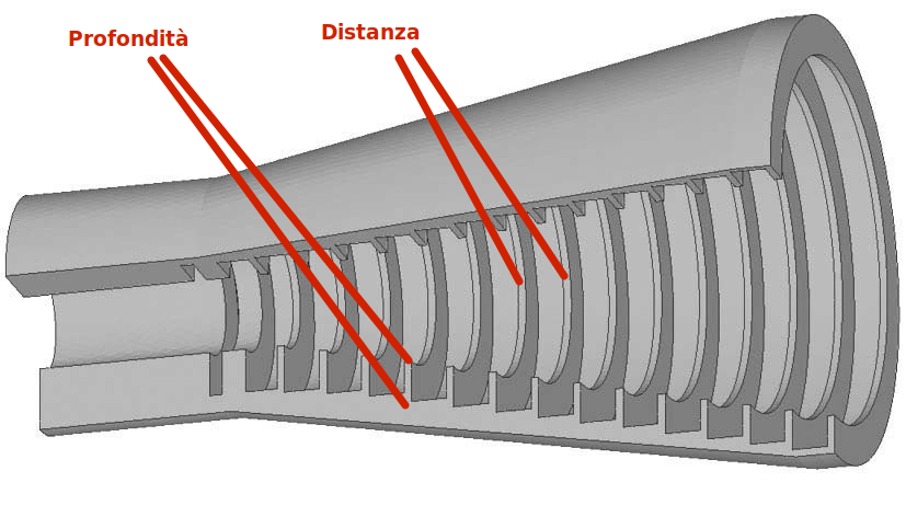
So every frequency we want to receive needs a horn that is built differently, or particular types of horn capable of receiving wide ranges of frequencies.
But why does the horn have this conical shape? The reason lies in what collects the radiation for the feed, namely the radio telescope. The radio electromagnetic radiation is collected and funnelled by the radio telescope into a cone-shaped beam, and to make sure that none of the collected radiation is lost, the mirror facing the horn must be entirely visible from the mouth of the horn — or, as we say, the horn must illuminate the mirror. For more details, see The radio telescope.
The radiation is thus guided by the waveguide at the entrance of the receiver down to the truly sensitive parts of the instrument, which absorb the energy of the radiation and turn it into an electric current.
Consider that the electrons inside the metal are free to move, and therefore do so in every possible direction within the metal bar. Once the radiation is funnelled by the horn towards the sensitive bars, the electrons in the metal bars begin to "feel" the effect of the wave's electric field. The electric field has a direction which, by convention, is the direction an electron would move if subjected to it. Looking at figure 3, for example, an electromagnetic wave travels from left to right, coming into contact with the metal bar represented by the vertical red line.
The electric field points downwards or upwards following the direction of the field of the incident wave. Inside the bar we thus obtain a current that for a very short time flows in one direction and for an equally short time in the opposite direction, following the frequency of the electromagnetic wave. A radio wave has a frequency ranging from about a hundred MHz up to nearly a thousand GHz — that is, it oscillates from about a hundred million to a thousand billion times per second. Likewise, the recorded current changes direction the same number of times per second.
An electromagnetic wave is characterised by a property called polarisation, which depends on how it was emitted by the astronomical source. For details on this property, see Polarisation of an electromagnetic wave.
To study this property of the radiation we split the signal into two parts — two polarisations, in fact — whose signals can then be combined to give further information about the phenomena that produced that radiation.
The sensitive parts of a front-end can be of two types, each of which serves to separate the two polarisations of the incident wave and to record them separately.
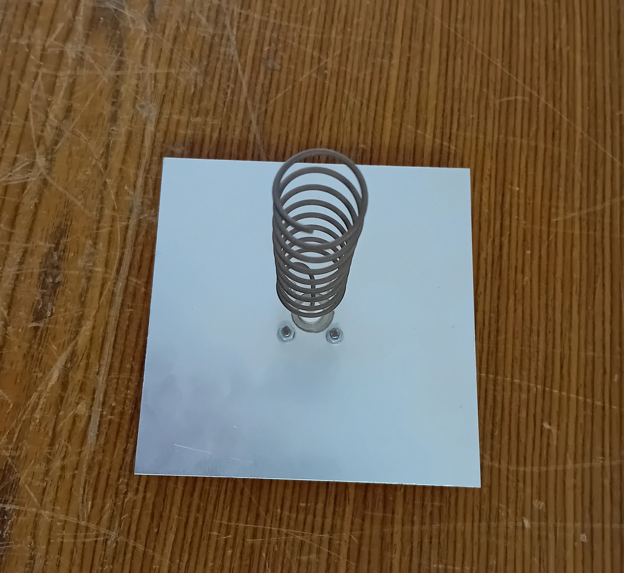
One possibility is the helical antenna, as in figure 4.
A helical antenna receives the wave that is circularly polarised (see Polarisation of an electromagnetic wave) in one direction of rotation. It has the shape of a spring, and the direction of rotation of the antenna determines which polarisation it will receive: running a finger along the antenna starting from the side exposed to the electromagnetic wave, if the finger turns clockwise the antenna receives right-hand circularly polarised electromagnetic waves, whereas if it winds anticlockwise it will receive left-hand circularly polarised waves. The incident wave is thus split into two waves, circularly polarised to the right and to the left.
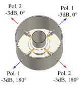
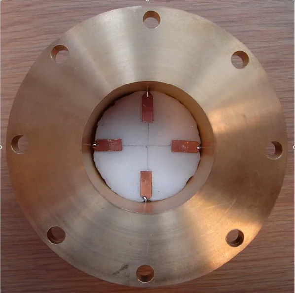
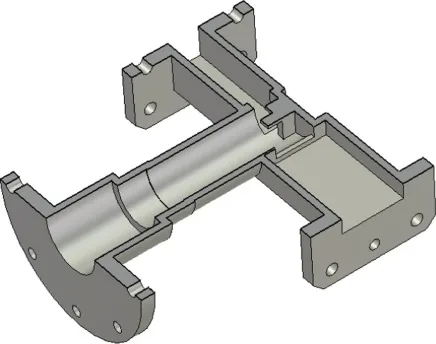
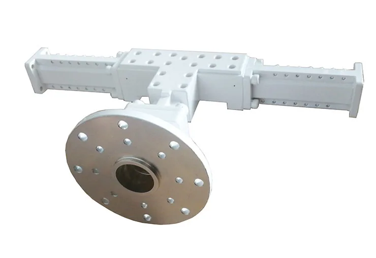
The most common antenna system consists of two metal bars perpendicular to each other placed at the end of the horn and across its axis (figures 5 and 6), or of one bar placed at each end of a beam splitter, called an orthomode transducer, which splits the wave into two linear polarisations, one perpendicular to the other (figures 7 and 8). We will see in the next section how these two linear polarisations are used.
The front-end then follows a scheme called superheterodyne, which serves an important purpose for the reception of radio transmissions in general, and of radio waves coming from astronomical objects in particular.
When you want to receive a radio signal you must select the frequency at which you want to receive it. Suppose we want to examine the radio emission of a radio galaxy at a frequency of 1.6 GHz. We say that the sky frequency or Radio Frequency (RF) at which we want to observe is, precisely, 1.6 GHz. Deciding at which frequency to observe matters for many reasons, which you can find in the section Observing in the radio band. To select only the emission at this frequency we need a filter that lets through only one band — an interval of frequencies — around the 1.6 GHz frequency, and we need an instrument that reads the power within that band. But if we then want to observe the same object at another sky frequency, say 22 GHz, besides the horn, as we have already seen, we would have to change both the filter and the reading instrument, because filtering and reading the power at two different frequencies requires differently built instruments. The superheterodyne system allows us to use a single instrument for filtering and reading, because the signal collected by the antenna, whatever its frequency, is converted into a signal at a frequency called the Intermediate Frequency (IF). As can be seen in fig. 9, the signal collected by the antenna is passed through a mixer and combined with a signal produced by an instrument called the local oscillator (LO).
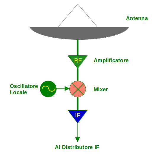
The frequency of the local oscillator can change according to the frequency we are observing. So if, for example, we want an IF of 1 GHz, we must subtract 0.6 GHz from the 1.6 GHz frequency and 21 GHz from the 22 GHz one. In both cases the sky frequency is mixed down by the local oscillator: for the first frequency the local oscillator will be at 0.6 GHz, while for the second its value will be 21 GHz. In both cases the IF will be the same, 1 GHz, allowing us to always use the same instrument for filtering and reading the signal. It is important to note that the power of the radiation does not change if we change its frequency, so the quality of the signal is not degraded.
Another important reason why the superheterodyne receiver was essential concerns the transfer of the signal from the receiver to the other instruments. Until a little more than a decade ago, the transport took place through waveguides, which have far greater losses at high frequencies. Converting the signal to a low frequency, typically around 500 MHz, was therefore also important to lose as little signal as possible.
Coming out of the mixer, the signal now passes through an optical converter that turns it into a signal that can be transmitted over optical fibre, which has absolutely negligible losses. It is then brought to the control room of the radio telescope, where it will pass through the IF distributor.
IF distributor
Once the signal has been "mixed" and its frequency converted to the intermediate frequency, it is transferred via optical fibre to the control room at the base of the radio telescope. Here an Intermediate Frequency (IF) distributor routes the signal to the instrumentation that will be used to analyse it.
The distributor receives the signal already converted into a current, amplifies it further and redirects it to the instrumentation along two separate lines: the two polarisations, right-hand circular and left-hand circular.
In the Front-end section we saw that the received radiation is split into two linear polarisations perpendicular to each other, yet we have just said that the polarisations are recorded as right-hand and left-hand circular. The use of circular polarisation (see Polarisation of an electromagnetic wave) originates in the reception of radio broadcasts.
A linear antenna only receives one polarisation, along the antenna itself, so if the polarisation of the transmission and the direction of the antenna do not match there would be reception problems. If the transmitted wave has circular polarisation, several million times per second the electric field of the wave will find itself parallel to the receiving antenna. That is why radio broadcasts always use a circularly polarised wave.
As we have seen, however, radio astronomy receivers record the two linear polarisations perpendicular to each other. How do we reconstruct a circular polarisation from two linear ones?
To understand it, we can look at fig. 10.
It shows how a circular trajectory can be composed of two linear motions. The vertical axis coincides with the oscillating motion of one small ball, the red one, while the horizontal axis is the one along which the blue ball oscillates. The green ball is the point where the vertical line through the blue ball meets the horizontal line through the red ball. Since the two motions are 90° out of phase — that is, when one ball is at zero the other is always at one of the points of maximum distance along its line — the combination of the two oscillations gives rise to a circle. In particular, it is a right-hand circular polarisation. By changing the phase difference we can produce a left-hand circular polarisation (fig. 8), or an elliptical motion of the green ball, or a linear motion (figs. 9 and 10).
In this way, by combining the signals recorded by each linear polariser we can reconstruct the two polarisations, right and left, and route them separately.
Back-end
The next element of the acquisition chain is the back-end, the instrument that prepares the signal so that it can be recorded. There are various back-ends, and their characteristics depend on the type of observation to be carried out. At the Noto Radio Astronomy Station we currently have two back-ends available.
DBBC
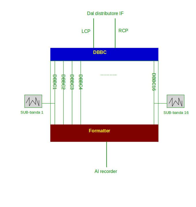
The Digital Base Band Converter (DBBC) is, as its name says, a digital base band converter. It is an instrument that acquires the band coming from the receivers through the IF distributor and converts it into digital form. As we have seen, the front-end is already a filter: it selects a range of radio frequencies from which it reads, amplifies and sends to the IF distributor the intensity of the radiation emitted by the observed source. The interval of frequencies transmitted by the receiver is called the receiver's passband. The whole band is sent as a block — that is, the information about how much radiation was collected at each frequency is all together in the signal arriving from the receiver.
In essence, each frequency travels through the waveguides and then through the optical fibre on its own, together with an intensity proportional to the intensity of the radiation that reached the radio telescope from the source. The back-end takes care of splitting this information into sub-bands, frequency intervals whose width is set according to the type of observation and what one wants to obtain. The scheme can be seen in fig. 14. The data stream arrives via optical fibre through the IF distributor at the DBBC; here the band is filtered into a certain number of sub-bands whose frequency and width are decided by the astronomers who requested the observation; finally, the formatter inside the DBBC creates the ordered stream of data that will be recorded in sequence on the storage medium, so that they can be retrieved in the same order when they are used.
Total power
This is a back-end for recording the intensity of the electromagnetic wave over a very wide band. This instrument integrates — that is, sums — the power arriving from the source in a band within the passband that the receiver can collect. This power is then converted into digital form and can be recorded as a signal in the form of a number, which can be converted into any physical unit useful to astronomers. We then have two modes for recording the data, corresponding to two modes of observation and hence of moving the antenna.
The first is the cross scan, an observing technique used to determine the flux of a source by sweeping the antenna across it in crossed passes. The other system is called on-off and, intuitively, is carried out by recording measurements on the source and off the source, in different directions. These observing techniques are usually employed, for example, to study the variability of a source over time, or to study its spectrum in the radio band — that is, how the brightness of the source varies as the observing frequency changes. The details of the two techniques are illustrated in the section Brightness measurements.
The Total Power back-end is also used for measurements based on the mapping technique, which is useful to obtain a radio image. The technique is described in detail in the section How do you take a picture in the radio band?.
Recorder
The data collected with the radio telescope must be recorded in some way so that they can later be reduced. In fact, no data on an astronomical source taken with a radio telescope can be used right away: it requires more or less complex operations to make it scientifically usable.
Let us start with the simplest mode, the one concerning the data collected through the Total Power back-end. In this case the data are just intensities tied to a position, so the recording is done on the same computer that manages the pointing of the radio telescope, and the data are simply written out in series to a text file. From this file, dedicated programs can produce plots useful for deriving the measurements relevant to the research being carried out. For example, as can be seen in the section Brightness measurements, plots of the radio flux measurements of the sources can be obtained, or the values derived from each measurement can be averaged to obtain more accurate estimates. For the data derived from mapping operations, the programs will be set up to reconstruct an image with isophotes or in false colours, as described in the section How do you take a picture in the radio band?.
Flexbuff
When interferometric data must be recorded (see the section The resolution problem in radio astronomy), a recording system is used that must take into account the requirements of that observing technique. This recorder is a computer running a specific program that receives the data already formatted by the DBBC.
The data coming from the DBBC have already been stamped with the timing information provided by the maser, and are therefore arranged to be recorded in a precise order — the same order in which they will be read during correlation, the final phase of an interferometric observation (see the section The resolution problem in radio astronomy).
The Flexbuff (fig. 15) is equipped with a set of solid-state disks, hence with very fast read speeds, needed to rapidly handle the amount of data being recorded.
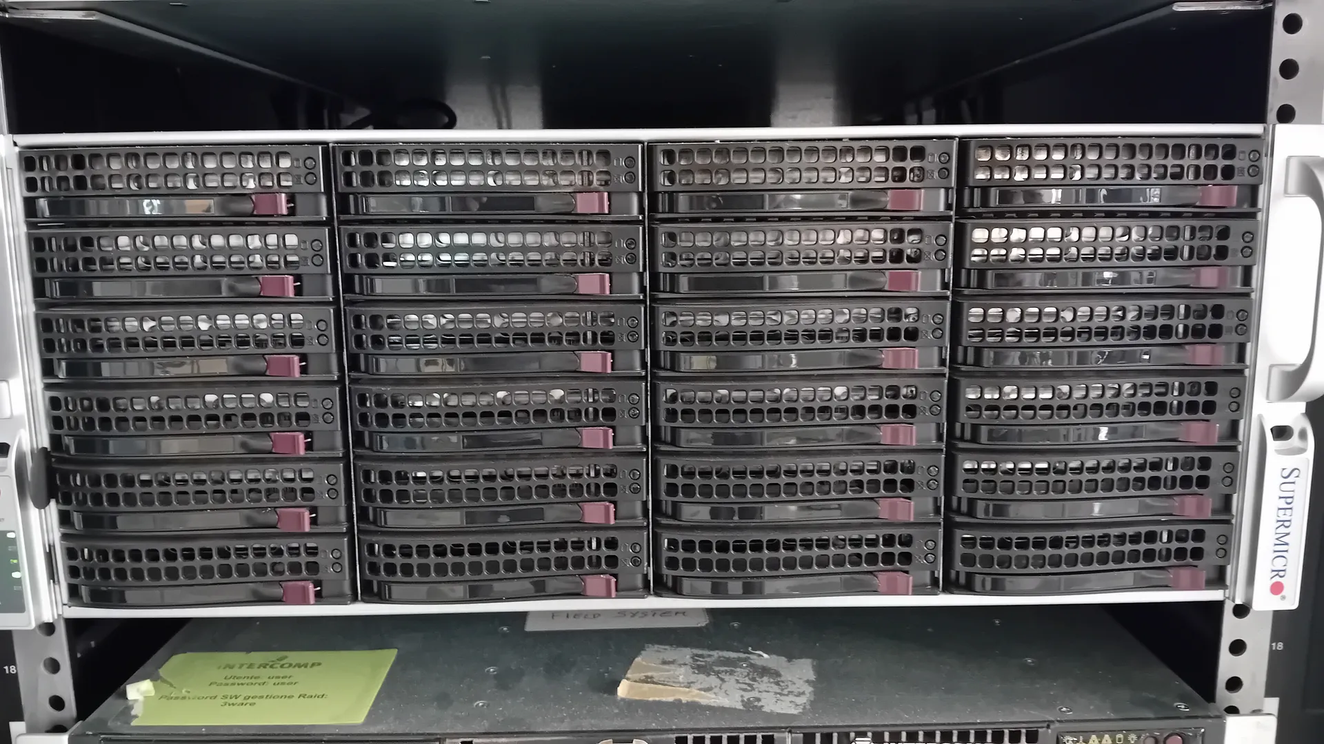
The total disk space is 400 TByte, which sounds like a lot — but only until you learn the speed at which the data are recorded. A Radio Astronomy Station of the European VLBI Network (see the section The resolution problem in radio astronomy) regularly records data at a speed of 1 Gb/s: this means that 1 GByte of data is recorded every 8 seconds. Moreover, we are already moving to twice that speed, and there are plans to reach 4 Gb/s, which would mean 1 GByte recorded every 2 seconds. And since an observation can go on for nearly 24 hours almost continuously, you can well understand that a substantial mass storage is needed. From the Flexbuff the data are then retrieved directly by the correlator in Dwingeloo, in the Netherlands, and processed to obtain the final data product that can be downloaded by the astronomers who requested the observation.
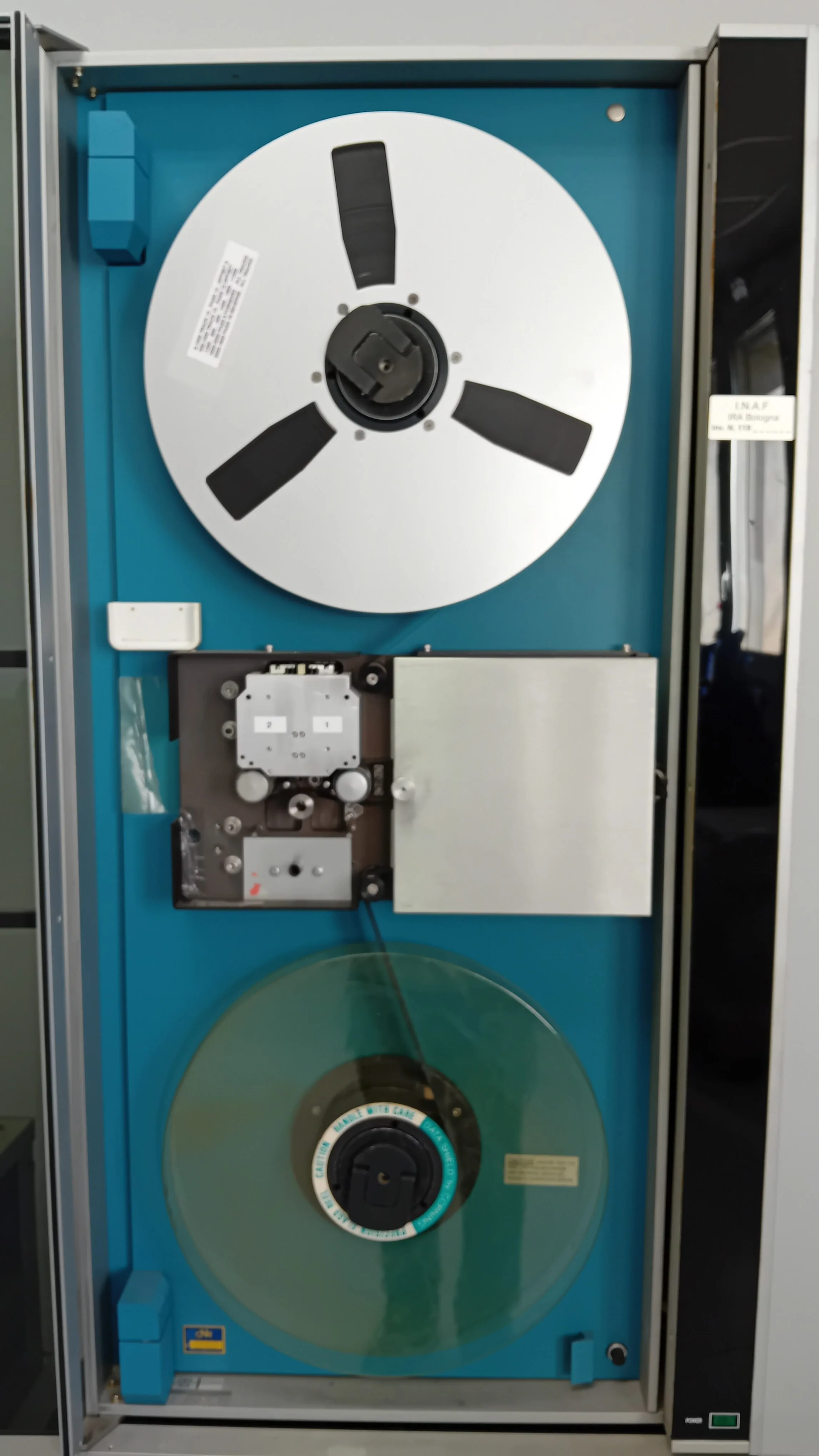
The recorder is the part that has evolved the most over the years. The great-great-grandfather of the Flexbuff is the video recorder, with video cassettes like the VHS tapes used for films, in use until about 2010 (fig. 16a).
Its capacity was decidedly limited. Then came the tapes (fig. 16b), which at first were enormous but not very capacious: each could hold only 15 minutes of observation, and since observations already lasted several hours back then, it was maddening to have to change tapes four times an hour, especially at night.
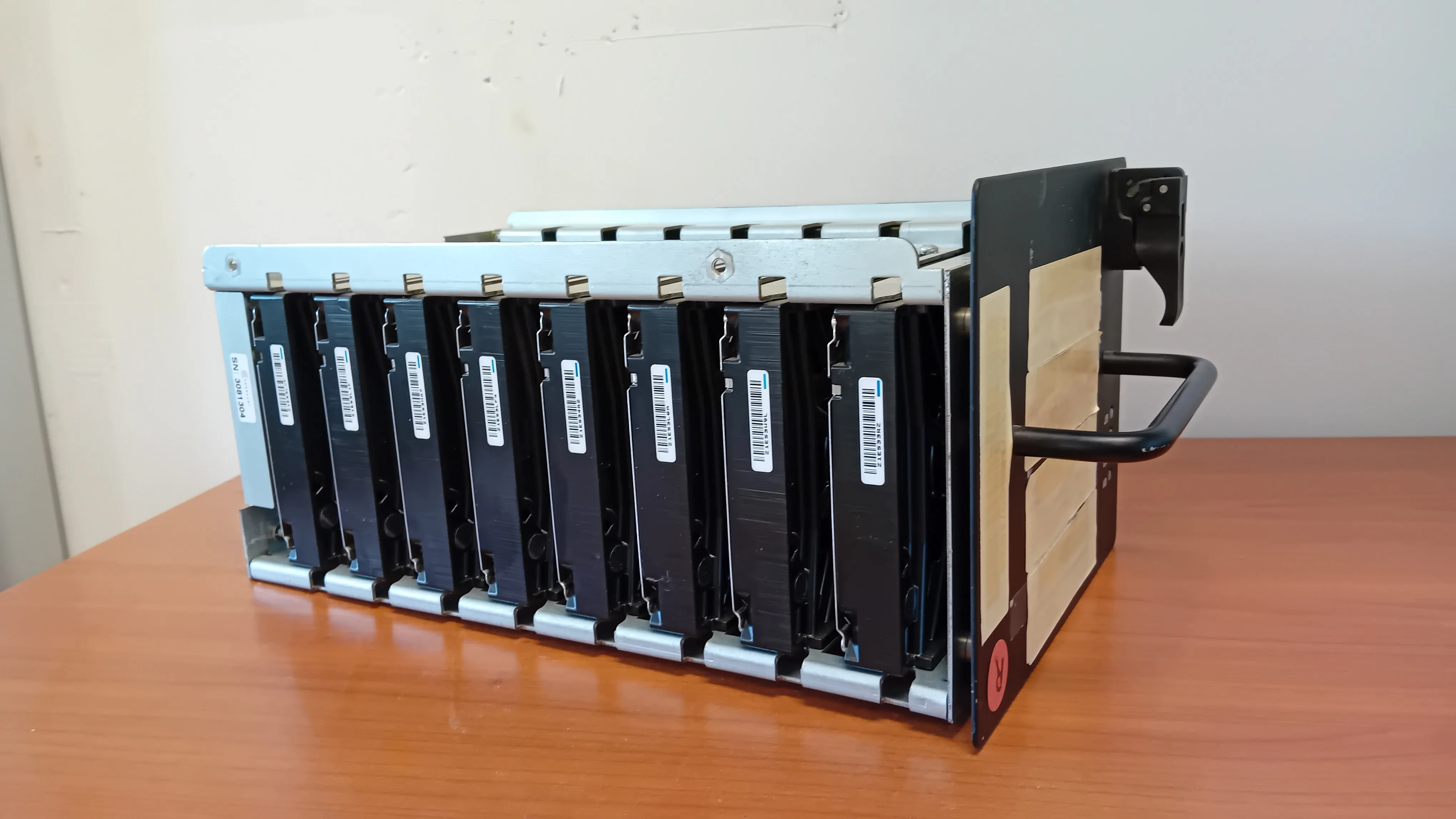
The capacity of the tapes grew thanks to more efficient recording systems and thinner tape, which made it possible to fit twice as many metres on the same reel. They came to hold about 500 GByte each. The next step was to record the data on hard drives like those used in computers, only arranged in packs of 8 suitably connected hard disks (fig. 16c).
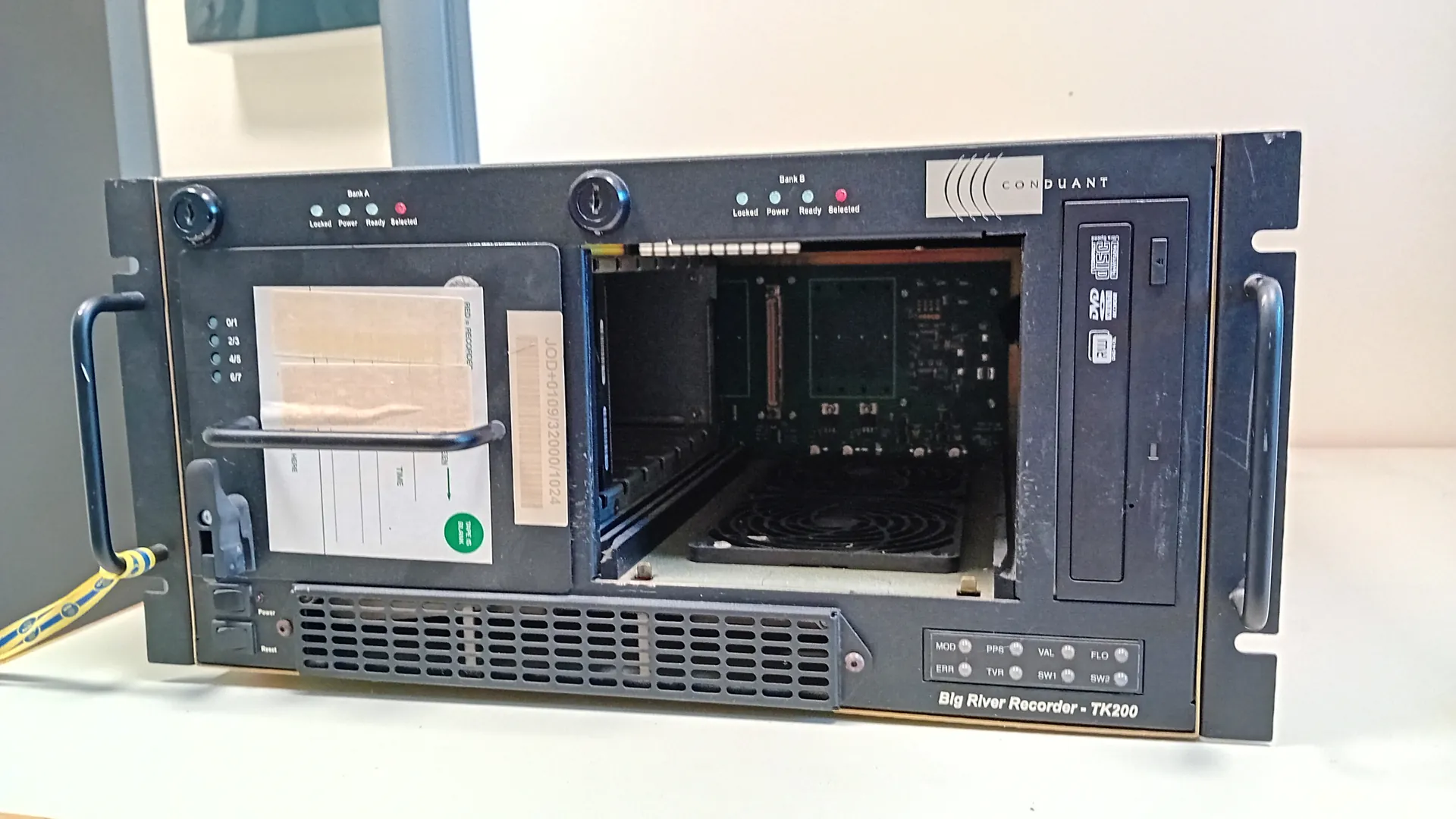
The disk packs were inserted into a purpose-built computer (fig. 16d) that recorded the data in a fuzzy mode, so that the information could be saved even if two out of eight hard disks failed. It started with twice the capacity of the tapes and ended with a capacity of 32 TByte per disk pack. As you can see, in all these cases the magnetic recording medium was removable. Indeed, the only system capable of effectively getting the data to the correlator was the postal service. There was no network fast enough to allow data transfer over the web. Now that the Noto Station is connected by fibre at a speed of 10 Gb/s, we can transfer enormous amounts of data in reasonable times. This allows the data to be recorded on non-removable media from which the correlator retrieves them directly over the network.